xclim: Software ecosystem for climate services
Author(s)
List authors, their current affiliations, up-to-date contact information, and ORCID if available. Add as many author lines as you need.
Author1 = {“name”: “Pascal Bourgault”, “affiliation”: “Ouranos Inc”, “email”: “bourgault.pascal@ouranos.ca”, “orcid”: “0000-0003-1192-0403”}
Author2 = {“name”: “Travis Logan”, “affiliation”: “Ouranos Inc”, “email”: “logan.travis@ouranos.ca”, “orcid”: “0000-0002-2212-9580”}
Author3 = {“name”: “David Huard”, “affiliation”: “Ouranos Inc”, “email”: “huard.david@ouranos.ca”, “orcid”: “0000-0003-0311-5498”}
Author4 = {“name”: “Trevor J. Smith”, “affiliation”: “Ouranos Inc”, “email”: “smith.trevorj@ouranos.ca”, “orcid”: “0000-0001-5393-8359”}
Table of Contents
Purpose
This notebook presents xclim, a python package allowing easy manipulation and analysis of N-D climate dataset. It goes in details on what tools xclim provides, and how it simplifies and standardizes climate analyses workflows. The notebook also demontrates how xclim functionality can be exposed as a Web Processing Service (WPS) through finch. This notebook was developped for Python 3.7+, but expects a special python environment and a running instance of finch. The configuration is optimized for running on binder.
Technical contributions
Development of a climate analysis library regrouping many different tools, with special attention to community standards (especially CF) and computationally efficient implementations.
Numerically efficient climate indices algorithms yielding standard-compliant outputs;
Model ensemble statistics and robustness metrics
Bias-adjustment algorithms
Other tools (not shown in this notebook) (subsetting, spatial analogs, calendar conversions)
Development of a web service exposing climate analysis processes through OGC’s WPS protocol.
Methodology
This notebook shows two examples of climate analysis workflows:
Calculating climate indices on an ensemble of simulation data, then computing ensemble statistics;
Bias-adjustment of model data.
Calculating climate indices through a web service (
finch).
The examples interleave code and markdown cells to describe what is being done. They also include some graphics created with holoviews, in order to give a clearer idea of what was achieved.
Results
This notebook demontrates how the use of xclim can help simplify and standardize climate analysis workflows.
Funding
This project benefitted from direct and indirect funding from multiple sources, which are cited in the “Acknowledgements” section below.
Keywords
keywords=[“climate”, “xarray”, “bias-adjustment”, “wps”]
Citation
Bourgault, Pascal et al. Ouranos, 2021. xclim: Software ecosystem for climate services. Accessed 2021/05/15 at https://github.com/Ouranosinc/xclim/blob/earthcube-nb/docs/notebooks/PB_01_xclim_Software_ecosystem_for_climate_services.ipynb
Suggested next steps
After reading through this notebook, we recommend looking at xclim’s documentation, especially the examples page, where other notebooks extend the examples shown here. Xclim offers other features that are not shown here, but might be of interest to readers : a spatial analogs submodule and internationalization utilities, among others. The list of indicators is also a good stop, and is regularly updated with new algorithms. It covers most indicators from ECAD to more complex and specialized one, like the Fire Weather Indexes.
The web service demontrated here is part of the bird-house ecosystem and project. It is used by different platforms, such as PAVICS and climatedata.ca.
Acknowledgements
Much of the development work of xclim was done to support climate services delivery at Ouranos and the Canadian Centre for Climate Services, and was funded by Environment and Climate Change Canada (ECCC). It has become a core component of the Power Analytics and Visualization for Climate Science (PAVICS) platform (Ouranos and CRIM 2021). PAVICS has been funded by CANARIE and the Québec Fonds Vert, and through other projects also benefits from the support of the Canadian Foundation for Innovation (CFI) and the Fonds de Recherche du Québec (FRQ). PAVICS is a joint effort of Ouranos and the Centre de Recherche en Informatique de Montréal (CRIM). xclim itself
Setup
Library import
import xclim
# Also import some submodules for direct access
import xclim.ensembles  # Ensemble creation and statistics
import xclim.sdba  # Bias-adjustment

# Data manipulation
import xarray as xr
import xclim.testing

# For interacting with finch WPS
import birdy

# Visualizations and display
from pprint import pprint
from IPython.display import display
import matplotlib as mpl
import matplotlib.pyplot as plt
from dask.diagnostics import ProgressBar

# For handling file paths
from pathlib import Path

# Some little figure tweaking
mpl.style.use('seaborn-deep')
mpl.style.use('seaborn-darkgrid')
%matplotlib inline
mpl.rcParams['figure.figsize'] = (12, 5)
Data import
In the first part, we use the “Ouranos standard ensemble of bias-adjusted climate scenarios version 1.0”, bias-adjusted and downscaled data from Ouranos. It includes 11 simulations from different climate models, all produced in the RCP8.5 experiment of the CMIP5 project. More information can be found on this page.
!du -hs data/*.nc
852K	data/ACCESS1-3_rcp85_singlept_1950-2100.nc
852K	data/BNU-ESM_rcp85_singlept_1950-2100.nc
852K	data/CanESM2_rcp85_singlept_1950-2100.nc
852K	data/CMCC-CMS_rcp85_singlept_1950-2100.nc
852K	data/GFDL-ESM2M_rcp85_singlept_1950-2100.nc
840K	data/HadGEM2-CC_rcp85_singlept_1950-2100.nc
852K	data/INM-CM4_rcp85_singlept_1950-2100.nc
848K	data/IPSL-CM5A-LR_rcp85_singlept_1950-2100.nc
848K	data/IPSL-CM5B-LR_rcp85_singlept_1950-2100.nc
852K	data/MPI-ESM-LR_rcp85_singlept_1950-2100.nc
852K	data/NorESM1-M_rcp85_singlept_1950-2100.nc
The second example, dealing with bias-adjustment, will use two sources. The model data comes from the CanESM2 model of CCCma. The reference time series are extracted from the Adjusted and Homogenized Canadian Climate Data (AHCCD), from Environment and Climate Change Canada. Both datasets are distributed under the Open Government Licence (Canada). We chose three weather stations representative of a reasonable range of climatic conditions and extracted time series over those locations from the model data.
Finally, the third section will use two datasets. A first one extracted from ECMWF’s ERA5 reanalysis includes time series extracted on a few locations for multiple variables. The second dataset is a subset of Natural Resources Canada (NRCAN)’s daily dataset derived from observational data. See https://cfs.nrcan.gc.ca/projects/3/4.
Data processing and analysis
Climate indices computation and ensemble statistics
A large part of climate data analytics is based on the computation and comparison of climate indices. Xclim’s main goal is to make it easier for researchers to process climate data and calculate those indices. It does so by providing a large library of climate indices, grouped in categories (CMIP’s “realms”) for convenience, but also by providing tools for all the small tweaks and pre- and post-processing steps that such workflows require.
xclim is built on xarray, which itself makes it easy to scale computations using dask. While many indices are conceptually simple, we aim to provide implementations that balance performance and code complexity. This allows for ease in understanding and extending the code base.
In the following steps we will use xclim to:
create an ensemble dataset,
compute a few climate indices,
calculate ensemble statistics on the results.
Creating the ensemble dataset
In xclim, an “ensemble dataset” is simply an xarray Dataset where multiple realizations of the same climate have been concatenated along a “realization” dimension. In our case here, as presented above, the realizations are in fact simulations from different models, but all have been bias-adjusted with the same reference. All ensemble-related functions are in the ensembles module.
Given a list of files, creating the ensemble dataset is straightforward:
# Get a list of files in the `earthcube_data`:
# The sort is not important here, it only ensures a consistent notebook output for automated checks
files = sorted(list(Path('data').glob('*1950-2100.nc')))

# Open files into the ensemble
ens = xclim.ensembles.create_ensemble(files)
ens
<xarray.Dataset>
Dimensions:      (realization: 11, time: 55152)
Coordinates:
  * time         (time) datetime64[ns] 1950-01-01 1950-01-02 ... 2100-12-31
    lat          float32 47.21
    lon          float32 -70.3
  * realization  (realization) int64 0 1 2 3 4 5 6 7 8 9 10
Data variables:
    pr           (realization, time) float32 dask.array<chunksize=(1, 55152), meta=np.ndarray>
    tasmax       (realization, time) float32 dask.array<chunksize=(1, 55152), meta=np.ndarray>
    tasmin       (realization, time) float32 dask.array<chunksize=(1, 55152), meta=np.ndarray>
Attributes:
    Conventions:     CF-1.5
    title:           ACCESS1-3 model output prepared for CMIP5 historical
    history:         CMIP5 compliant file produced from raw ACCESS model outp...
    institution:     CSIRO (Commonwealth Scientific and Industrial Research O...
    source:          ACCESS1-3 2011. Atmosphere: AGCM v1.0 (N96 grid-point, 1...
redistribution: Redistribution prohibited. For internal use only.- realization: 11
- time: 55152
- time(time)datetime64[ns]1950-01-01 ... 2100-12-31
- axis :
- T
- long_name :
- time
- standard_name :
- time
array(['1950-01-01T00:00:00.000000000', '1950-01-02T00:00:00.000000000', '1950-01-03T00:00:00.000000000', ..., '2100-12-29T00:00:00.000000000', '2100-12-30T00:00:00.000000000', '2100-12-31T00:00:00.000000000'], dtype='datetime64[ns]') - lat()float3247.21
- axis :
- Y
- units :
- degrees_north
- long_name :
- latitude
- standard_name :
- latitude
array(47.20742, dtype=float32)
- lon()float32-70.3
- axis :
- X
- units :
- degrees_east
- long_name :
- longitude
- standard_name :
- longitude
array(-70.29596, dtype=float32)
- realization(realization)int640 1 2 3 4 5 6 7 8 9 10
- axis :
- E
array([ 0, 1, 2, 3, 4, 5, 6, 7, 8, 9, 10])
- pr(realization, time)float32dask.array<chunksize=(1, 55152), meta=np.ndarray>
- units :
- mm s-1
- long_name :
- lwe_precipitation_rate
- standard_name :
- lwe_precipitation_rate
Array Chunk Bytes 2.31 MiB 215.44 kiB Shape (11, 55152) (1, 55152) Count 85 Tasks 11 Chunks Type float32 numpy.ndarray - tasmax(realization, time)float32dask.array<chunksize=(1, 55152), meta=np.ndarray>
- units :
- K
- long_name :
- air_temperature
- standard_name :
- air_temperature
Array Chunk Bytes 2.31 MiB 215.44 kiB Shape (11, 55152) (1, 55152) Count 85 Tasks 11 Chunks Type float32 numpy.ndarray - tasmin(realization, time)float32dask.array<chunksize=(1, 55152), meta=np.ndarray>
- units :
- K
- long_name :
- air_temperature
- standard_name :
- air_temperature
Array Chunk Bytes 2.31 MiB 215.44 kiB Shape (11, 55152) (1, 55152) Count 85 Tasks 11 Chunks Type float32 numpy.ndarray
- Conventions :
- CF-1.5
- title :
- ACCESS1-3 model output prepared for CMIP5 historical
- history :
- CMIP5 compliant file produced from raw ACCESS model output using the ACCESS Post-Processor and CMOR2. 2012-04-03T13:44:54Z CMOR rewrote data to comply with CF standards and CMIP5 requirements. Fri Apr 13 09:55:30 2012: forcing attribute modified to correct value Fri Apr 13 12:29:45 2012: corrected model_id from ACCESS1-3 to ACCESS1.3 Mon Jul 2 11:13:41 2012: updated version number to v20120413. 2016-01-19T03:26:16: Interpolate to nrcan_livneh grid. 2016-02-10T09:50:00: Bias correction using nrcan_livneh.
- institution :
- CSIRO (Commonwealth Scientific and Industrial Research Organisation, Australia), and BOM (Bureau of Meteorology, Australia)
- source :
- ACCESS1-3 2011. Atmosphere: AGCM v1.0 (N96 grid-point, 1.875 degrees EW x approx 1.25 degree NS, 38 levels); ocean: NOAA/GFDL MOM4p1 (nominal 1.0 degree EW x 1.0 degrees NS, tripolar north of 65N, equatorial refinement to 1/3 degree from 10S to 10 N, cosine dependent NS south of 25S, 50 levels); sea ice: CICE4.1 (nominal 1.0 degree EW x 1.0 degrees NS, tripolar north of 65N, equatorial refinement to 1/3 degree from 10S to 10 N, cosine dependent NS south of 25S); land: CABLE1.0 (1.875 degree EW x 1.25 degree NS, 6 levels 30-day moving window 50-bins quantile mapping with detrending.
- redistribution :
- Redistribution prohibited. For internal use only.
(Note: similarly to xarray.open_mfdataset, used internally, the dataset attributes are actually from the first file only.)
But how is this different from xarray.concat(files, concat_dim='realization)? While only slighlty more shorter to write, the main difference is the handling of incompatible calendars. Different models often use different calendars and this causes issues when merging/concatening their data in xarray. Xclim provides xclim.core.calendar.convert_calendar to handle this. For example, in this ensemble, we have a simulation of the HadGEM2 model which uses the “360_day” calendar:
ds360 = xr.open_dataset('data/HadGEM2-CC_rcp85_singlept_1950-2100.nc')
ds360.time[59].data
array(cftime.Datetime360Day(1950, 2, 30, 0, 0, 0, 0), dtype=object)
# Convert to the `noleap` calendar, see doc for details on arguments.
ds365 = xclim.core.calendar.convert_calendar(ds360, 'noleap', align_on='date')
ds365.time[59].data
array(cftime.DatetimeNoLeap(1950, 3, 2, 0, 0, 0, 0), dtype=object)
This conversion dropped the invalid days (for example: the 29th and 30th of February 1950) and convert the dtype of the time axis. This does alter the data, but it makes it possible to concatenate different model simulations into a single DataArray.
In create_ensemble, all members are converted to a common calendar. By default, it uses the normal numpy/pandas data type (a range-limited calendar equivalent to proleptic_gregorian), but for this model ensemble, it’s better to use noleap (all years have 365 days), as it is the calendar used in most models included here.
ens = xclim.ensembles.create_ensemble(files, calendar='noleap')
ens
<xarray.Dataset>
Dimensions:      (realization: 11, time: 55115)
Coordinates:
  * time         (time) object 1950-01-01 00:00:00 ... 2100-12-31 00:00:00
    lat          float32 47.21
    lon          float32 -70.3
  * realization  (realization) int64 0 1 2 3 4 5 6 7 8 9 10
Data variables:
    pr           (realization, time) float32 dask.array<chunksize=(1, 55115), meta=np.ndarray>
    tasmax       (realization, time) float32 dask.array<chunksize=(1, 55115), meta=np.ndarray>
    tasmin       (realization, time) float32 dask.array<chunksize=(1, 55115), meta=np.ndarray>
Attributes:
    Conventions:     CF-1.5
    title:           ACCESS1-3 model output prepared for CMIP5 historical
    history:         CMIP5 compliant file produced from raw ACCESS model outp...
    institution:     CSIRO (Commonwealth Scientific and Industrial Research O...
    source:          ACCESS1-3 2011. Atmosphere: AGCM v1.0 (N96 grid-point, 1...
redistribution: Redistribution prohibited. For internal use only.- realization: 11
- time: 55115
- time(time)object1950-01-01 00:00:00 ... 2100-12-...
- axis :
- T
- long_name :
- time
- standard_name :
- time
array([cftime.DatetimeNoLeap(1950, 1, 1, 0, 0, 0, 0), cftime.DatetimeNoLeap(1950, 1, 2, 0, 0, 0, 0), cftime.DatetimeNoLeap(1950, 1, 3, 0, 0, 0, 0), ..., cftime.DatetimeNoLeap(2100, 12, 29, 0, 0, 0, 0), cftime.DatetimeNoLeap(2100, 12, 30, 0, 0, 0, 0), cftime.DatetimeNoLeap(2100, 12, 31, 0, 0, 0, 0)], dtype=object) - lat()float3247.21
- axis :
- Y
- units :
- degrees_north
- long_name :
- latitude
- standard_name :
- latitude
array(47.20742, dtype=float32)
- lon()float32-70.3
- axis :
- X
- units :
- degrees_east
- long_name :
- longitude
- standard_name :
- longitude
array(-70.29596, dtype=float32)
- realization(realization)int640 1 2 3 4 5 6 7 8 9 10
- axis :
- E
array([ 0, 1, 2, 3, 4, 5, 6, 7, 8, 9, 10])
- pr(realization, time)float32dask.array<chunksize=(1, 55115), meta=np.ndarray>
- units :
- mm s-1
- long_name :
- lwe_precipitation_rate
- standard_name :
- lwe_precipitation_rate
Array Chunk Bytes 2.31 MiB 215.29 kiB Shape (11, 55115) (1, 55115) Count 63 Tasks 11 Chunks Type float32 numpy.ndarray - tasmax(realization, time)float32dask.array<chunksize=(1, 55115), meta=np.ndarray>
- units :
- K
- long_name :
- air_temperature
- standard_name :
- air_temperature
Array Chunk Bytes 2.31 MiB 215.29 kiB Shape (11, 55115) (1, 55115) Count 63 Tasks 11 Chunks Type float32 numpy.ndarray - tasmin(realization, time)float32dask.array<chunksize=(1, 55115), meta=np.ndarray>
- units :
- K
- long_name :
- air_temperature
- standard_name :
- air_temperature
Array Chunk Bytes 2.31 MiB 215.29 kiB Shape (11, 55115) (1, 55115) Count 63 Tasks 11 Chunks Type float32 numpy.ndarray
- Conventions :
- CF-1.5
- title :
- ACCESS1-3 model output prepared for CMIP5 historical
- history :
- CMIP5 compliant file produced from raw ACCESS model output using the ACCESS Post-Processor and CMOR2. 2012-04-03T13:44:54Z CMOR rewrote data to comply with CF standards and CMIP5 requirements. Fri Apr 13 09:55:30 2012: forcing attribute modified to correct value Fri Apr 13 12:29:45 2012: corrected model_id from ACCESS1-3 to ACCESS1.3 Mon Jul 2 11:13:41 2012: updated version number to v20120413. 2016-01-19T03:26:16: Interpolate to nrcan_livneh grid. 2016-02-10T09:50:00: Bias correction using nrcan_livneh.
- institution :
- CSIRO (Commonwealth Scientific and Industrial Research Organisation, Australia), and BOM (Bureau of Meteorology, Australia)
- source :
- ACCESS1-3 2011. Atmosphere: AGCM v1.0 (N96 grid-point, 1.875 degrees EW x approx 1.25 degree NS, 38 levels); ocean: NOAA/GFDL MOM4p1 (nominal 1.0 degree EW x 1.0 degrees NS, tripolar north of 65N, equatorial refinement to 1/3 degree from 10S to 10 N, cosine dependent NS south of 25S, 50 levels); sea ice: CICE4.1 (nominal 1.0 degree EW x 1.0 degrees NS, tripolar north of 65N, equatorial refinement to 1/3 degree from 10S to 10 N, cosine dependent NS south of 25S); land: CABLE1.0 (1.875 degree EW x 1.25 degree NS, 6 levels 30-day moving window 50-bins quantile mapping with detrending.
- redistribution :
- Redistribution prohibited. For internal use only.
Compute climate indicators
Climate indicators are stored in xclim.indicators.[realm] and act as functions, taking xarray.DataArray as input variables and returning one (or more) DataArray. Most indicators also take keyword arguments to control various parameters. Under the hood, indicators are python objects, storing information on what the computation does, its inputs and its outputs. For example, let’s look at the tropical_nights indicator:
TN = xclim.indicators.atmos.tropical_nights

# Print general information:
print('Title: ', TN.title)
print('General description: ', TN.abstract, '\n')

# Info on the inputs
print('Inputs description:')
pprint(TN.parameters)
print()

# Info on the output
print('Output description:')
pprint(TN.cf_attrs)
Title:  Tropical nights.
General description:  The number of days with minimum daily temperature above threshold.

Inputs description:
{'ds': {'default': None,
        'description': 'A dataset with the variables given by name.',
        'kind': <InputKind.DATASET: 70>},
 'freq': {'default': 'YS',
          'description': 'Resampling frequency.',
          'kind': <InputKind.FREQ_STR: 3>},
 'tasmin': {'default': 'tasmin',
            'description': 'Minimum daily temperature.',
            'kind': <InputKind.VARIABLE: 0>,
            'units': '[temperature]'},
 'thresh': {'default': '20.0 degC',
            'description': 'Threshold temperature on which to base evaluation.',
            'kind': <InputKind.QUANTITY_STR: 2>,
            'units': '[temperature]'}}

Output description:
[{'cell_methods': 'time: minimum within days time: sum over days',
  'description': '{freq} number of Tropical Nights : defined as days with '
                 'minimum daily temperature above {thresh}',
  'long_name': 'Number of Tropical Nights (Tmin > {thresh})',
  'standard_name': 'number_of_days_with_air_temperature_above_threshold',
  'units': 'days',
  'var_name': 'tropical_nights'}]
We use the indicator by calling it like a function with the variable and parameters. We will look at the seasonal number of “tropical nights” with a threshold of 5°C. For frequency arguments, we use the same syntax as pandas. Here QS-DEC will resample to seasons of three (3) months, starting in December (so DJF, MMA, JJA, SON).
out = xclim.indicators.atmos.tropical_nights(tasmin=ens.tasmin, thresh='5 degC', freq='QS-DEC')
display(out.data)
out.isel(time=slice(0, 2)).load()
/home/phobos/.conda/envs/xclim-demo/lib/python3.9/site-packages/xclim/indicators/atmos/_temperature.py:83: UserWarning: Variable does not have a `cell_methods` attribute.
  cfchecks.check_valid(tasmin, "cell_methods", "*time: minimum within days*")
|
<xarray.DataArray 'tropical_nights' (realization: 11, time: 2)>
array([[nan,  9.],
       [nan,  9.],
       [nan, 15.],
       [nan, 15.],
       [nan,  9.],
       [nan, nan],
       [nan, 12.],
       [nan,  2.],
       [nan, 20.],
       [nan, 15.],
       [nan, 17.]])
Coordinates:
  * time         (time) object 1949-12-01 00:00:00 1950-03-01 00:00:00
    lat          float32 47.21
    lon          float32 -70.3
  * realization  (realization) int64 0 1 2 3 4 5 6 7 8 9 10
Attributes:
    units:          days
    cell_methods:    time: minimum within days time: sum over days
    xclim_history:  [2021-06-07 17:30:27] tropical_nights: TROPICAL_NIGHTS(ta...
    standard_name:  number_of_days_with_air_temperature_above_threshold
    long_name:      Number of tropical nights (tmin > 5 degc)
description: Seasonal number of tropical nights : defined as days with...- realization: 11
- time: 2
- nan 9.0 nan 9.0 nan 15.0 nan 15.0 ... 2.0 nan 20.0 nan 15.0 nan 17.0
array([[nan, 9.], [nan, 9.], [nan, 15.], [nan, 15.], [nan, 9.], [nan, nan], [nan, 12.], [nan, 2.], [nan, 20.], [nan, 15.], [nan, 17.]]) - time(time)object1949-12-01 00:00:00 1950-03-01 0...
array([cftime.DatetimeNoLeap(1949, 12, 1, 0, 0, 0, 0), cftime.DatetimeNoLeap(1950, 3, 1, 0, 0, 0, 0)], dtype=object) - lat()float3247.21
- axis :
- Y
- units :
- degrees_north
- long_name :
- latitude
- standard_name :
- latitude
array(47.20742, dtype=float32)
- lon()float32-70.3
- axis :
- X
- units :
- degrees_east
- long_name :
- longitude
- standard_name :
- longitude
array(-70.29596, dtype=float32)
- realization(realization)int640 1 2 3 4 5 6 7 8 9 10
- axis :
- E
array([ 0, 1, 2, 3, 4, 5, 6, 7, 8, 9, 10])
- units :
- days
- cell_methods :
- time: minimum within days time: sum over days
- xclim_history :
- [2021-06-07 17:30:27] tropical_nights: TROPICAL_NIGHTS(tasmin=<array>, thresh='5 degC', freq='QS-DEC') - xclim version: 0.26.1.
- standard_name :
- number_of_days_with_air_temperature_above_threshold
- long_name :
- Number of tropical nights (tmin > 5 degc)
- description :
- Seasonal number of tropical nights : defined as days with minimum daily temperature above 5 degc
Let’s talk about the many things that happened here:
Input checks
Before the real computation, xclim performs some checks on the inputs. These can differ between indicators, but the most common are CF convention and input frequency checks. The former looks at the
standard_nameandcell_methodsattributes of the input variable and raises warnings when they do not fit with what it expects. Here, thestandard_name(“air_temperature”) is correct, but the variable is missing thecell_methodsattribute that would normally indicate that this is indeed the minimum temperature within each days.The second type of checks looks at the data itself. Most indicators expect data at a daily frequency, and if the input has a different frequency, the indicator checks will raise an error.
Unit handling
Another check on the inputs is performed to ensure the correct units were passed. Above, in the
parametersdictionary, we saw thattropical_nightsexpectstasminandthreshto both be “[temperature]” values. In the function, conversion are made to ensure compatible units. Here,tasminis in Kelvin andthreshwas given in Celsius. Under the hood, xclim usespintto handle this, but with small modifications made so that CF-compliant unit strings are understood.Missing values handling
After the computation, for indicators involving a resampling operation, periods where at least one value was missing (i.e. was a
np.NaN) are masked out. Here the first period is masked for all realization since there was no data for the month of december 1949. This is the default behavior and it can be changed, as we will show further down.Metadata formatting
The output’s attributes were formatted to include some information from the passed parameters. Notice how the description includes the given threshold and frequency (Seasonal number of tropical nights […]).
Lazy computing
This is not a feature inherent to xclim, but, by default,
create_ensemblewill open the ensemble dataset using thedaskbackend, one “chunk” for each file. This means that all further calculations are lazy, ie: python remembers the operations but doesn’t perform them as long as the result is not requested. This is why we needed to call.load()to see the first values of the output. This behaviour fromxarrayis extremely useful for computationally-intensive workflows as it allowsdaskto efficiently manage the memory and CPU ressources. Xclim aims to implement its indicators in a lazy and efficient way.
Let’s compute a few indicators and merge them into another ensemble dataset. This time, we will change the missing values handling to a more relaxed method, where periods are masked when at least 5% of the elements are missing. Moreover, we will set an option so that CF-checks warnings are ignored.
If you want to know more about the indicators we are computing, you can use help(indicator) or indicator? (in ipython/jupyter) to print their docstrings, which include most information shown above.
# Set options using a "context". Options set here are reset to their defaults as soon as we exit the "with" block
with xclim.set_options(cf_compliance='log', check_missing='pct', missing_options={'pct': {'tolerance': 0.05}}):

    # Intermediate computation : Approximate mean daily temp by taking the mean of tasmin and tasmax
    tas = xclim.indicators.atmos.tg(tasmin=ens.tasmin, tasmax=ens.tasmax)

    # First day below, first day of the year where tasmin goes below "thresh" for at least "window" days
    # Note that we resample yearly, but starting in July, so that the full winter is included
    out_fda = xclim.indicators.atmos.first_day_below(tasmin=ens.tasmin, thresh='-5 degC', window=3, freq='AS-JUL')

    # Number frost days : total number of days where tasmin < 0 degC
    out_nfd = xclim.indicators.atmos.frost_days(tasmin=ens.tasmin, freq='AS-JUL')

    # Solid precipitation accumulation : total thickness of solid precipitation (estimated by pr when tas < 0°C)
    out_spa = xclim.indicators.atmos.solid_precip_accumulation(pr=ens.pr, tas=tas, freq='AS-JUL')

    # Cold spell freq : Number of spells where tas is under "thresh" for at least "window" days.
    out_csf = xclim.indicators.atmos.cold_spell_frequency(tas=tas, thresh='-10 degC', window=3, freq='AS-JUL')

out = xr.merge([out_fda, out_nfd, out_spa, out_csf])
out
<xarray.Dataset>
Dimensions:               (realization: 11, time: 152)
Coordinates:
  * time                  (time) object 1949-07-01 00:00:00 ... 2100-07-01 00...
    lat                   float32 47.21
    lon                   float32 -70.3
  * realization           (realization) int64 0 1 2 3 4 5 6 7 8 9 10
Data variables:
    first_day_below       (realization, time) float64 dask.array<chunksize=(1, 1), meta=np.ndarray>
    frost_days            (realization, time) float64 dask.array<chunksize=(1, 1), meta=np.ndarray>
    solidprcptot          (realization, time) float64 dask.array<chunksize=(1, 1), meta=np.ndarray>
    cold_spell_frequency  (realization, time) float64 dask.array<chunksize=(1, 1), meta=np.ndarray>
Attributes:
    units:
    is_dayofyear:   1
    calendar:       noleap
    cell_methods:
    xclim_history:  [2021-06-07 17:30:33] first_day_below: FIRST_DAY_BELOW(ta...
    standard_name:  day_of_year
    long_name:      First day of year with temperature below -5 degc
description: First day of year with temperature below -5 degc for at l...- realization: 11
- time: 152
- time(time)object1949-07-01 00:00:00 ... 2100-07-...
array([cftime.DatetimeNoLeap(1949, 7, 1, 0, 0, 0, 0), cftime.DatetimeNoLeap(1950, 7, 1, 0, 0, 0, 0), cftime.DatetimeNoLeap(1951, 7, 1, 0, 0, 0, 0), cftime.DatetimeNoLeap(1952, 7, 1, 0, 0, 0, 0), cftime.DatetimeNoLeap(1953, 7, 1, 0, 0, 0, 0), cftime.DatetimeNoLeap(1954, 7, 1, 0, 0, 0, 0), cftime.DatetimeNoLeap(1955, 7, 1, 0, 0, 0, 0), cftime.DatetimeNoLeap(1956, 7, 1, 0, 0, 0, 0), cftime.DatetimeNoLeap(1957, 7, 1, 0, 0, 0, 0), cftime.DatetimeNoLeap(1958, 7, 1, 0, 0, 0, 0), cftime.DatetimeNoLeap(1959, 7, 1, 0, 0, 0, 0), cftime.DatetimeNoLeap(1960, 7, 1, 0, 0, 0, 0), cftime.DatetimeNoLeap(1961, 7, 1, 0, 0, 0, 0), cftime.DatetimeNoLeap(1962, 7, 1, 0, 0, 0, 0), cftime.DatetimeNoLeap(1963, 7, 1, 0, 0, 0, 0), cftime.DatetimeNoLeap(1964, 7, 1, 0, 0, 0, 0), cftime.DatetimeNoLeap(1965, 7, 1, 0, 0, 0, 0), cftime.DatetimeNoLeap(1966, 7, 1, 0, 0, 0, 0), cftime.DatetimeNoLeap(1967, 7, 1, 0, 0, 0, 0), cftime.DatetimeNoLeap(1968, 7, 1, 0, 0, 0, 0), cftime.DatetimeNoLeap(1969, 7, 1, 0, 0, 0, 0), cftime.DatetimeNoLeap(1970, 7, 1, 0, 0, 0, 0), cftime.DatetimeNoLeap(1971, 7, 1, 0, 0, 0, 0), cftime.DatetimeNoLeap(1972, 7, 1, 0, 0, 0, 0), cftime.DatetimeNoLeap(1973, 7, 1, 0, 0, 0, 0), cftime.DatetimeNoLeap(1974, 7, 1, 0, 0, 0, 0), cftime.DatetimeNoLeap(1975, 7, 1, 0, 0, 0, 0), cftime.DatetimeNoLeap(1976, 7, 1, 0, 0, 0, 0), cftime.DatetimeNoLeap(1977, 7, 1, 0, 0, 0, 0), cftime.DatetimeNoLeap(1978, 7, 1, 0, 0, 0, 0), cftime.DatetimeNoLeap(1979, 7, 1, 0, 0, 0, 0), cftime.DatetimeNoLeap(1980, 7, 1, 0, 0, 0, 0), cftime.DatetimeNoLeap(1981, 7, 1, 0, 0, 0, 0), cftime.DatetimeNoLeap(1982, 7, 1, 0, 0, 0, 0), cftime.DatetimeNoLeap(1983, 7, 1, 0, 0, 0, 0), cftime.DatetimeNoLeap(1984, 7, 1, 0, 0, 0, 0), cftime.DatetimeNoLeap(1985, 7, 1, 0, 0, 0, 0), cftime.DatetimeNoLeap(1986, 7, 1, 0, 0, 0, 0), cftime.DatetimeNoLeap(1987, 7, 1, 0, 0, 0, 0), cftime.DatetimeNoLeap(1988, 7, 1, 0, 0, 0, 0), cftime.DatetimeNoLeap(1989, 7, 1, 0, 0, 0, 0), cftime.DatetimeNoLeap(1990, 7, 1, 0, 0, 0, 0), cftime.DatetimeNoLeap(1991, 7, 1, 0, 0, 0, 0), cftime.DatetimeNoLeap(1992, 7, 1, 0, 0, 0, 0), cftime.DatetimeNoLeap(1993, 7, 1, 0, 0, 0, 0), cftime.DatetimeNoLeap(1994, 7, 1, 0, 0, 0, 0), cftime.DatetimeNoLeap(1995, 7, 1, 0, 0, 0, 0), cftime.DatetimeNoLeap(1996, 7, 1, 0, 0, 0, 0), cftime.DatetimeNoLeap(1997, 7, 1, 0, 0, 0, 0), cftime.DatetimeNoLeap(1998, 7, 1, 0, 0, 0, 0), cftime.DatetimeNoLeap(1999, 7, 1, 0, 0, 0, 0), cftime.DatetimeNoLeap(2000, 7, 1, 0, 0, 0, 0), cftime.DatetimeNoLeap(2001, 7, 1, 0, 0, 0, 0), cftime.DatetimeNoLeap(2002, 7, 1, 0, 0, 0, 0), cftime.DatetimeNoLeap(2003, 7, 1, 0, 0, 0, 0), cftime.DatetimeNoLeap(2004, 7, 1, 0, 0, 0, 0), cftime.DatetimeNoLeap(2005, 7, 1, 0, 0, 0, 0), cftime.DatetimeNoLeap(2006, 7, 1, 0, 0, 0, 0), cftime.DatetimeNoLeap(2007, 7, 1, 0, 0, 0, 0), cftime.DatetimeNoLeap(2008, 7, 1, 0, 0, 0, 0), cftime.DatetimeNoLeap(2009, 7, 1, 0, 0, 0, 0), cftime.DatetimeNoLeap(2010, 7, 1, 0, 0, 0, 0), cftime.DatetimeNoLeap(2011, 7, 1, 0, 0, 0, 0), cftime.DatetimeNoLeap(2012, 7, 1, 0, 0, 0, 0), cftime.DatetimeNoLeap(2013, 7, 1, 0, 0, 0, 0), cftime.DatetimeNoLeap(2014, 7, 1, 0, 0, 0, 0), cftime.DatetimeNoLeap(2015, 7, 1, 0, 0, 0, 0), cftime.DatetimeNoLeap(2016, 7, 1, 0, 0, 0, 0), cftime.DatetimeNoLeap(2017, 7, 1, 0, 0, 0, 0), cftime.DatetimeNoLeap(2018, 7, 1, 0, 0, 0, 0), cftime.DatetimeNoLeap(2019, 7, 1, 0, 0, 0, 0), cftime.DatetimeNoLeap(2020, 7, 1, 0, 0, 0, 0), cftime.DatetimeNoLeap(2021, 7, 1, 0, 0, 0, 0), cftime.DatetimeNoLeap(2022, 7, 1, 0, 0, 0, 0), cftime.DatetimeNoLeap(2023, 7, 1, 0, 0, 0, 0), cftime.DatetimeNoLeap(2024, 7, 1, 0, 0, 0, 0), cftime.DatetimeNoLeap(2025, 7, 1, 0, 0, 0, 0), cftime.DatetimeNoLeap(2026, 7, 1, 0, 0, 0, 0), cftime.DatetimeNoLeap(2027, 7, 1, 0, 0, 0, 0), cftime.DatetimeNoLeap(2028, 7, 1, 0, 0, 0, 0), cftime.DatetimeNoLeap(2029, 7, 1, 0, 0, 0, 0), cftime.DatetimeNoLeap(2030, 7, 1, 0, 0, 0, 0), cftime.DatetimeNoLeap(2031, 7, 1, 0, 0, 0, 0), cftime.DatetimeNoLeap(2032, 7, 1, 0, 0, 0, 0), cftime.DatetimeNoLeap(2033, 7, 1, 0, 0, 0, 0), cftime.DatetimeNoLeap(2034, 7, 1, 0, 0, 0, 0), cftime.DatetimeNoLeap(2035, 7, 1, 0, 0, 0, 0), cftime.DatetimeNoLeap(2036, 7, 1, 0, 0, 0, 0), cftime.DatetimeNoLeap(2037, 7, 1, 0, 0, 0, 0), cftime.DatetimeNoLeap(2038, 7, 1, 0, 0, 0, 0), cftime.DatetimeNoLeap(2039, 7, 1, 0, 0, 0, 0), cftime.DatetimeNoLeap(2040, 7, 1, 0, 0, 0, 0), cftime.DatetimeNoLeap(2041, 7, 1, 0, 0, 0, 0), cftime.DatetimeNoLeap(2042, 7, 1, 0, 0, 0, 0), cftime.DatetimeNoLeap(2043, 7, 1, 0, 0, 0, 0), cftime.DatetimeNoLeap(2044, 7, 1, 0, 0, 0, 0), cftime.DatetimeNoLeap(2045, 7, 1, 0, 0, 0, 0), cftime.DatetimeNoLeap(2046, 7, 1, 0, 0, 0, 0), cftime.DatetimeNoLeap(2047, 7, 1, 0, 0, 0, 0), cftime.DatetimeNoLeap(2048, 7, 1, 0, 0, 0, 0), cftime.DatetimeNoLeap(2049, 7, 1, 0, 0, 0, 0), cftime.DatetimeNoLeap(2050, 7, 1, 0, 0, 0, 0), cftime.DatetimeNoLeap(2051, 7, 1, 0, 0, 0, 0), cftime.DatetimeNoLeap(2052, 7, 1, 0, 0, 0, 0), cftime.DatetimeNoLeap(2053, 7, 1, 0, 0, 0, 0), cftime.DatetimeNoLeap(2054, 7, 1, 0, 0, 0, 0), cftime.DatetimeNoLeap(2055, 7, 1, 0, 0, 0, 0), cftime.DatetimeNoLeap(2056, 7, 1, 0, 0, 0, 0), cftime.DatetimeNoLeap(2057, 7, 1, 0, 0, 0, 0), cftime.DatetimeNoLeap(2058, 7, 1, 0, 0, 0, 0), cftime.DatetimeNoLeap(2059, 7, 1, 0, 0, 0, 0), cftime.DatetimeNoLeap(2060, 7, 1, 0, 0, 0, 0), cftime.DatetimeNoLeap(2061, 7, 1, 0, 0, 0, 0), cftime.DatetimeNoLeap(2062, 7, 1, 0, 0, 0, 0), cftime.DatetimeNoLeap(2063, 7, 1, 0, 0, 0, 0), cftime.DatetimeNoLeap(2064, 7, 1, 0, 0, 0, 0), cftime.DatetimeNoLeap(2065, 7, 1, 0, 0, 0, 0), cftime.DatetimeNoLeap(2066, 7, 1, 0, 0, 0, 0), cftime.DatetimeNoLeap(2067, 7, 1, 0, 0, 0, 0), cftime.DatetimeNoLeap(2068, 7, 1, 0, 0, 0, 0), cftime.DatetimeNoLeap(2069, 7, 1, 0, 0, 0, 0), cftime.DatetimeNoLeap(2070, 7, 1, 0, 0, 0, 0), cftime.DatetimeNoLeap(2071, 7, 1, 0, 0, 0, 0), cftime.DatetimeNoLeap(2072, 7, 1, 0, 0, 0, 0), cftime.DatetimeNoLeap(2073, 7, 1, 0, 0, 0, 0), cftime.DatetimeNoLeap(2074, 7, 1, 0, 0, 0, 0), cftime.DatetimeNoLeap(2075, 7, 1, 0, 0, 0, 0), cftime.DatetimeNoLeap(2076, 7, 1, 0, 0, 0, 0), cftime.DatetimeNoLeap(2077, 7, 1, 0, 0, 0, 0), cftime.DatetimeNoLeap(2078, 7, 1, 0, 0, 0, 0), cftime.DatetimeNoLeap(2079, 7, 1, 0, 0, 0, 0), cftime.DatetimeNoLeap(2080, 7, 1, 0, 0, 0, 0), cftime.DatetimeNoLeap(2081, 7, 1, 0, 0, 0, 0), cftime.DatetimeNoLeap(2082, 7, 1, 0, 0, 0, 0), cftime.DatetimeNoLeap(2083, 7, 1, 0, 0, 0, 0), cftime.DatetimeNoLeap(2084, 7, 1, 0, 0, 0, 0), cftime.DatetimeNoLeap(2085, 7, 1, 0, 0, 0, 0), cftime.DatetimeNoLeap(2086, 7, 1, 0, 0, 0, 0), cftime.DatetimeNoLeap(2087, 7, 1, 0, 0, 0, 0), cftime.DatetimeNoLeap(2088, 7, 1, 0, 0, 0, 0), cftime.DatetimeNoLeap(2089, 7, 1, 0, 0, 0, 0), cftime.DatetimeNoLeap(2090, 7, 1, 0, 0, 0, 0), cftime.DatetimeNoLeap(2091, 7, 1, 0, 0, 0, 0), cftime.DatetimeNoLeap(2092, 7, 1, 0, 0, 0, 0), cftime.DatetimeNoLeap(2093, 7, 1, 0, 0, 0, 0), cftime.DatetimeNoLeap(2094, 7, 1, 0, 0, 0, 0), cftime.DatetimeNoLeap(2095, 7, 1, 0, 0, 0, 0), cftime.DatetimeNoLeap(2096, 7, 1, 0, 0, 0, 0), cftime.DatetimeNoLeap(2097, 7, 1, 0, 0, 0, 0), cftime.DatetimeNoLeap(2098, 7, 1, 0, 0, 0, 0), cftime.DatetimeNoLeap(2099, 7, 1, 0, 0, 0, 0), cftime.DatetimeNoLeap(2100, 7, 1, 0, 0, 0, 0)], dtype=object) - lat()float3247.21
- axis :
- Y
- units :
- degrees_north
- long_name :
- latitude
- standard_name :
- latitude
array(47.20742, dtype=float32)
- lon()float32-70.3
- axis :
- X
- units :
- degrees_east
- long_name :
- longitude
- standard_name :
- longitude
array(-70.29596, dtype=float32)
- realization(realization)int640 1 2 3 4 5 6 7 8 9 10
- axis :
- E
array([ 0, 1, 2, 3, 4, 5, 6, 7, 8, 9, 10])
- first_day_below(realization, time)float64dask.array<chunksize=(1, 1), meta=np.ndarray>
- units :
- is_dayofyear :
- 1
- calendar :
- noleap
- cell_methods :
- xclim_history :
- [2021-06-07 17:30:33] first_day_below: FIRST_DAY_BELOW(tasmin=<array>, thresh='-5 degC', after_date='07-01', window=3, freq='AS-JUL') - xclim version: 0.26.1.
- standard_name :
- day_of_year
- long_name :
- First day of year with temperature below -5 degc
- description :
- First day of year with temperature below -5 degc for at least 3 days.
Array Chunk Bytes 13.06 kiB 8 B Shape (11, 152) (1, 1) Count 75835 Tasks 1672 Chunks Type float64 numpy.ndarray - frost_days(realization, time)float64dask.array<chunksize=(1, 1), meta=np.ndarray>
- units :
- days
- cell_methods :
- time: minimum within days time: sum over days
- xclim_history :
- [2021-06-07 17:30:41] frost_days: FROST_DAYS(tasmin=<array>, thresh='0 degC', freq='AS-JUL') - xclim version: 0.26.1.
- standard_name :
- days_with_air_temperature_below_threshold
- long_name :
- Number of frost days (tmin < 0c)
- description :
- Annual number of days with minimum daily temperature below 0℃.
Array Chunk Bytes 13.06 kiB 8 B Shape (11, 152) (1, 1) Count 45677 Tasks 1672 Chunks Type float64 numpy.ndarray - solidprcptot(realization, time)float64dask.array<chunksize=(1, 1), meta=np.ndarray>
- units :
- mm
- cell_methods :
- tas: time: mean within days time: sum within days time: sum over days
- xclim_history :
- pr: tas: [2021-06-07 17:30:43] solidprcptot: SOLIDPRCPTOT(pr=<array>, tas=<array>, thresh='0 degC', freq='AS-JUL', phase='solid') - xclim version: 0.26.1.
- standard_name :
- lwe_thickness_of_snowfall_amount
- long_name :
- Total solid precipitation
- description :
- Annual total solid precipitation, estimated as precipitation when temperature < 0 degc
Array Chunk Bytes 13.06 kiB 8 B Shape (11, 152) (1, 1) Count 64229 Tasks 1672 Chunks Type float64 numpy.ndarray - cold_spell_frequency(realization, time)float64dask.array<chunksize=(1, 1), meta=np.ndarray>
- units :
- cell_methods :
- time: mean within days
- xclim_history :
- [2021-06-07 17:30:46] cold_spell_frequency: COLD_SPELL_FREQUENCY(tas=<array>, thresh='-10 degC', window=3, freq='AS-JUL') - xclim version: 0.26.1.
- standard_name :
- cold_spell_frequency
- long_name :
- Number of cold spell events
- description :
- Annual number cold spell events, defined as 3 or more consecutive days with mean daily temperature below -10 degc.
Array Chunk Bytes 13.06 kiB 8 B Shape (11, 152) (1, 1) Count 47418 Tasks 1672 Chunks Type float64 numpy.ndarray
- units :
- is_dayofyear :
- 1
- calendar :
- noleap
- cell_methods :
- xclim_history :
- [2021-06-07 17:30:33] first_day_below: FIRST_DAY_BELOW(tasmin=<array>, thresh='-5 degC', after_date='07-01', window=3, freq='AS-JUL') - xclim version: 0.26.1.
- standard_name :
- day_of_year
- long_name :
- First day of year with temperature below -5 degc
- description :
- First day of year with temperature below -5 degc for at least 3 days.
Ensemble statistics
All this is quite cool, but we still have a large amount of data to manage. In order to get an idea of the climatic evolution of our indicators and of the model uncertainty associated with it, we can compute ensemble percentiles. Here we extract the 10th, 50th (median) and 90th percentile of the distribution made up of the 11 members of the ensemble.
out_perc = xclim.ensembles.ensemble_percentiles(out, values=[10, 50, 90], split=False)
out_perc
<xarray.Dataset>
Dimensions:               (percentiles: 3, time: 152)
Coordinates:
  * time                  (time) object 1949-07-01 00:00:00 ... 2100-07-01 00...
    lat                   float32 47.21
    lon                   float32 -70.3
  * percentiles           (percentiles) int64 10 50 90
Data variables:
    first_day_below       (time, percentiles) float64 dask.array<chunksize=(1, 3), meta=np.ndarray>
    frost_days            (time, percentiles) float64 dask.array<chunksize=(1, 3), meta=np.ndarray>
    solidprcptot          (time, percentiles) float64 dask.array<chunksize=(1, 3), meta=np.ndarray>
    cold_spell_frequency  (time, percentiles) float64 dask.array<chunksize=(1, 3), meta=np.ndarray>
Attributes:
    units:
    is_dayofyear:   1
    calendar:       noleap
    cell_methods:
    xclim_history:  [2021-06-07 17:30:48] : Computation of the percentiles on...
    standard_name:  day_of_year
    long_name:      First day of year with temperature below -5 degc
description: First day of year with temperature below -5 degc for at l...- percentiles: 3
- time: 152
- time(time)object1949-07-01 00:00:00 ... 2100-07-...
array([cftime.DatetimeNoLeap(1949, 7, 1, 0, 0, 0, 0), cftime.DatetimeNoLeap(1950, 7, 1, 0, 0, 0, 0), cftime.DatetimeNoLeap(1951, 7, 1, 0, 0, 0, 0), cftime.DatetimeNoLeap(1952, 7, 1, 0, 0, 0, 0), cftime.DatetimeNoLeap(1953, 7, 1, 0, 0, 0, 0), cftime.DatetimeNoLeap(1954, 7, 1, 0, 0, 0, 0), cftime.DatetimeNoLeap(1955, 7, 1, 0, 0, 0, 0), cftime.DatetimeNoLeap(1956, 7, 1, 0, 0, 0, 0), cftime.DatetimeNoLeap(1957, 7, 1, 0, 0, 0, 0), cftime.DatetimeNoLeap(1958, 7, 1, 0, 0, 0, 0), cftime.DatetimeNoLeap(1959, 7, 1, 0, 0, 0, 0), cftime.DatetimeNoLeap(1960, 7, 1, 0, 0, 0, 0), cftime.DatetimeNoLeap(1961, 7, 1, 0, 0, 0, 0), cftime.DatetimeNoLeap(1962, 7, 1, 0, 0, 0, 0), cftime.DatetimeNoLeap(1963, 7, 1, 0, 0, 0, 0), cftime.DatetimeNoLeap(1964, 7, 1, 0, 0, 0, 0), cftime.DatetimeNoLeap(1965, 7, 1, 0, 0, 0, 0), cftime.DatetimeNoLeap(1966, 7, 1, 0, 0, 0, 0), cftime.DatetimeNoLeap(1967, 7, 1, 0, 0, 0, 0), cftime.DatetimeNoLeap(1968, 7, 1, 0, 0, 0, 0), cftime.DatetimeNoLeap(1969, 7, 1, 0, 0, 0, 0), cftime.DatetimeNoLeap(1970, 7, 1, 0, 0, 0, 0), cftime.DatetimeNoLeap(1971, 7, 1, 0, 0, 0, 0), cftime.DatetimeNoLeap(1972, 7, 1, 0, 0, 0, 0), cftime.DatetimeNoLeap(1973, 7, 1, 0, 0, 0, 0), cftime.DatetimeNoLeap(1974, 7, 1, 0, 0, 0, 0), cftime.DatetimeNoLeap(1975, 7, 1, 0, 0, 0, 0), cftime.DatetimeNoLeap(1976, 7, 1, 0, 0, 0, 0), cftime.DatetimeNoLeap(1977, 7, 1, 0, 0, 0, 0), cftime.DatetimeNoLeap(1978, 7, 1, 0, 0, 0, 0), cftime.DatetimeNoLeap(1979, 7, 1, 0, 0, 0, 0), cftime.DatetimeNoLeap(1980, 7, 1, 0, 0, 0, 0), cftime.DatetimeNoLeap(1981, 7, 1, 0, 0, 0, 0), cftime.DatetimeNoLeap(1982, 7, 1, 0, 0, 0, 0), cftime.DatetimeNoLeap(1983, 7, 1, 0, 0, 0, 0), cftime.DatetimeNoLeap(1984, 7, 1, 0, 0, 0, 0), cftime.DatetimeNoLeap(1985, 7, 1, 0, 0, 0, 0), cftime.DatetimeNoLeap(1986, 7, 1, 0, 0, 0, 0), cftime.DatetimeNoLeap(1987, 7, 1, 0, 0, 0, 0), cftime.DatetimeNoLeap(1988, 7, 1, 0, 0, 0, 0), cftime.DatetimeNoLeap(1989, 7, 1, 0, 0, 0, 0), cftime.DatetimeNoLeap(1990, 7, 1, 0, 0, 0, 0), cftime.DatetimeNoLeap(1991, 7, 1, 0, 0, 0, 0), cftime.DatetimeNoLeap(1992, 7, 1, 0, 0, 0, 0), cftime.DatetimeNoLeap(1993, 7, 1, 0, 0, 0, 0), cftime.DatetimeNoLeap(1994, 7, 1, 0, 0, 0, 0), cftime.DatetimeNoLeap(1995, 7, 1, 0, 0, 0, 0), cftime.DatetimeNoLeap(1996, 7, 1, 0, 0, 0, 0), cftime.DatetimeNoLeap(1997, 7, 1, 0, 0, 0, 0), cftime.DatetimeNoLeap(1998, 7, 1, 0, 0, 0, 0), cftime.DatetimeNoLeap(1999, 7, 1, 0, 0, 0, 0), cftime.DatetimeNoLeap(2000, 7, 1, 0, 0, 0, 0), cftime.DatetimeNoLeap(2001, 7, 1, 0, 0, 0, 0), cftime.DatetimeNoLeap(2002, 7, 1, 0, 0, 0, 0), cftime.DatetimeNoLeap(2003, 7, 1, 0, 0, 0, 0), cftime.DatetimeNoLeap(2004, 7, 1, 0, 0, 0, 0), cftime.DatetimeNoLeap(2005, 7, 1, 0, 0, 0, 0), cftime.DatetimeNoLeap(2006, 7, 1, 0, 0, 0, 0), cftime.DatetimeNoLeap(2007, 7, 1, 0, 0, 0, 0), cftime.DatetimeNoLeap(2008, 7, 1, 0, 0, 0, 0), cftime.DatetimeNoLeap(2009, 7, 1, 0, 0, 0, 0), cftime.DatetimeNoLeap(2010, 7, 1, 0, 0, 0, 0), cftime.DatetimeNoLeap(2011, 7, 1, 0, 0, 0, 0), cftime.DatetimeNoLeap(2012, 7, 1, 0, 0, 0, 0), cftime.DatetimeNoLeap(2013, 7, 1, 0, 0, 0, 0), cftime.DatetimeNoLeap(2014, 7, 1, 0, 0, 0, 0), cftime.DatetimeNoLeap(2015, 7, 1, 0, 0, 0, 0), cftime.DatetimeNoLeap(2016, 7, 1, 0, 0, 0, 0), cftime.DatetimeNoLeap(2017, 7, 1, 0, 0, 0, 0), cftime.DatetimeNoLeap(2018, 7, 1, 0, 0, 0, 0), cftime.DatetimeNoLeap(2019, 7, 1, 0, 0, 0, 0), cftime.DatetimeNoLeap(2020, 7, 1, 0, 0, 0, 0), cftime.DatetimeNoLeap(2021, 7, 1, 0, 0, 0, 0), cftime.DatetimeNoLeap(2022, 7, 1, 0, 0, 0, 0), cftime.DatetimeNoLeap(2023, 7, 1, 0, 0, 0, 0), cftime.DatetimeNoLeap(2024, 7, 1, 0, 0, 0, 0), cftime.DatetimeNoLeap(2025, 7, 1, 0, 0, 0, 0), cftime.DatetimeNoLeap(2026, 7, 1, 0, 0, 0, 0), cftime.DatetimeNoLeap(2027, 7, 1, 0, 0, 0, 0), cftime.DatetimeNoLeap(2028, 7, 1, 0, 0, 0, 0), cftime.DatetimeNoLeap(2029, 7, 1, 0, 0, 0, 0), cftime.DatetimeNoLeap(2030, 7, 1, 0, 0, 0, 0), cftime.DatetimeNoLeap(2031, 7, 1, 0, 0, 0, 0), cftime.DatetimeNoLeap(2032, 7, 1, 0, 0, 0, 0), cftime.DatetimeNoLeap(2033, 7, 1, 0, 0, 0, 0), cftime.DatetimeNoLeap(2034, 7, 1, 0, 0, 0, 0), cftime.DatetimeNoLeap(2035, 7, 1, 0, 0, 0, 0), cftime.DatetimeNoLeap(2036, 7, 1, 0, 0, 0, 0), cftime.DatetimeNoLeap(2037, 7, 1, 0, 0, 0, 0), cftime.DatetimeNoLeap(2038, 7, 1, 0, 0, 0, 0), cftime.DatetimeNoLeap(2039, 7, 1, 0, 0, 0, 0), cftime.DatetimeNoLeap(2040, 7, 1, 0, 0, 0, 0), cftime.DatetimeNoLeap(2041, 7, 1, 0, 0, 0, 0), cftime.DatetimeNoLeap(2042, 7, 1, 0, 0, 0, 0), cftime.DatetimeNoLeap(2043, 7, 1, 0, 0, 0, 0), cftime.DatetimeNoLeap(2044, 7, 1, 0, 0, 0, 0), cftime.DatetimeNoLeap(2045, 7, 1, 0, 0, 0, 0), cftime.DatetimeNoLeap(2046, 7, 1, 0, 0, 0, 0), cftime.DatetimeNoLeap(2047, 7, 1, 0, 0, 0, 0), cftime.DatetimeNoLeap(2048, 7, 1, 0, 0, 0, 0), cftime.DatetimeNoLeap(2049, 7, 1, 0, 0, 0, 0), cftime.DatetimeNoLeap(2050, 7, 1, 0, 0, 0, 0), cftime.DatetimeNoLeap(2051, 7, 1, 0, 0, 0, 0), cftime.DatetimeNoLeap(2052, 7, 1, 0, 0, 0, 0), cftime.DatetimeNoLeap(2053, 7, 1, 0, 0, 0, 0), cftime.DatetimeNoLeap(2054, 7, 1, 0, 0, 0, 0), cftime.DatetimeNoLeap(2055, 7, 1, 0, 0, 0, 0), cftime.DatetimeNoLeap(2056, 7, 1, 0, 0, 0, 0), cftime.DatetimeNoLeap(2057, 7, 1, 0, 0, 0, 0), cftime.DatetimeNoLeap(2058, 7, 1, 0, 0, 0, 0), cftime.DatetimeNoLeap(2059, 7, 1, 0, 0, 0, 0), cftime.DatetimeNoLeap(2060, 7, 1, 0, 0, 0, 0), cftime.DatetimeNoLeap(2061, 7, 1, 0, 0, 0, 0), cftime.DatetimeNoLeap(2062, 7, 1, 0, 0, 0, 0), cftime.DatetimeNoLeap(2063, 7, 1, 0, 0, 0, 0), cftime.DatetimeNoLeap(2064, 7, 1, 0, 0, 0, 0), cftime.DatetimeNoLeap(2065, 7, 1, 0, 0, 0, 0), cftime.DatetimeNoLeap(2066, 7, 1, 0, 0, 0, 0), cftime.DatetimeNoLeap(2067, 7, 1, 0, 0, 0, 0), cftime.DatetimeNoLeap(2068, 7, 1, 0, 0, 0, 0), cftime.DatetimeNoLeap(2069, 7, 1, 0, 0, 0, 0), cftime.DatetimeNoLeap(2070, 7, 1, 0, 0, 0, 0), cftime.DatetimeNoLeap(2071, 7, 1, 0, 0, 0, 0), cftime.DatetimeNoLeap(2072, 7, 1, 0, 0, 0, 0), cftime.DatetimeNoLeap(2073, 7, 1, 0, 0, 0, 0), cftime.DatetimeNoLeap(2074, 7, 1, 0, 0, 0, 0), cftime.DatetimeNoLeap(2075, 7, 1, 0, 0, 0, 0), cftime.DatetimeNoLeap(2076, 7, 1, 0, 0, 0, 0), cftime.DatetimeNoLeap(2077, 7, 1, 0, 0, 0, 0), cftime.DatetimeNoLeap(2078, 7, 1, 0, 0, 0, 0), cftime.DatetimeNoLeap(2079, 7, 1, 0, 0, 0, 0), cftime.DatetimeNoLeap(2080, 7, 1, 0, 0, 0, 0), cftime.DatetimeNoLeap(2081, 7, 1, 0, 0, 0, 0), cftime.DatetimeNoLeap(2082, 7, 1, 0, 0, 0, 0), cftime.DatetimeNoLeap(2083, 7, 1, 0, 0, 0, 0), cftime.DatetimeNoLeap(2084, 7, 1, 0, 0, 0, 0), cftime.DatetimeNoLeap(2085, 7, 1, 0, 0, 0, 0), cftime.DatetimeNoLeap(2086, 7, 1, 0, 0, 0, 0), cftime.DatetimeNoLeap(2087, 7, 1, 0, 0, 0, 0), cftime.DatetimeNoLeap(2088, 7, 1, 0, 0, 0, 0), cftime.DatetimeNoLeap(2089, 7, 1, 0, 0, 0, 0), cftime.DatetimeNoLeap(2090, 7, 1, 0, 0, 0, 0), cftime.DatetimeNoLeap(2091, 7, 1, 0, 0, 0, 0), cftime.DatetimeNoLeap(2092, 7, 1, 0, 0, 0, 0), cftime.DatetimeNoLeap(2093, 7, 1, 0, 0, 0, 0), cftime.DatetimeNoLeap(2094, 7, 1, 0, 0, 0, 0), cftime.DatetimeNoLeap(2095, 7, 1, 0, 0, 0, 0), cftime.DatetimeNoLeap(2096, 7, 1, 0, 0, 0, 0), cftime.DatetimeNoLeap(2097, 7, 1, 0, 0, 0, 0), cftime.DatetimeNoLeap(2098, 7, 1, 0, 0, 0, 0), cftime.DatetimeNoLeap(2099, 7, 1, 0, 0, 0, 0), cftime.DatetimeNoLeap(2100, 7, 1, 0, 0, 0, 0)], dtype=object) - lat()float3247.21
- axis :
- Y
- units :
- degrees_north
- long_name :
- latitude
- standard_name :
- latitude
array(47.20742, dtype=float32)
- lon()float32-70.3
- axis :
- X
- units :
- degrees_east
- long_name :
- longitude
- standard_name :
- longitude
array(-70.29596, dtype=float32)
- percentiles(percentiles)int6410 50 90
array([10, 50, 90])
- first_day_below(time, percentiles)float64dask.array<chunksize=(1, 3), meta=np.ndarray>
- units :
- is_dayofyear :
- 1
- calendar :
- noleap
- cell_methods :
- xclim_history :
- [2021-06-07 17:30:48] : Computation of the percentiles on 11 ensemble members. - xclim version: 0.26.1.
- standard_name :
- day_of_year
- long_name :
- First day of year with temperature below -5 degc
- description :
- First day of year with temperature below -5 degc for at least 3 days.
Array Chunk Bytes 3.56 kiB 24 B Shape (152, 3) (1, 3) Count 76595 Tasks 152 Chunks Type float64 numpy.ndarray - frost_days(time, percentiles)float64dask.array<chunksize=(1, 3), meta=np.ndarray>
- units :
- days
- cell_methods :
- time: minimum within days time: sum over days
- xclim_history :
- [2021-06-07 17:30:48] : Computation of the percentiles on 11 ensemble members. - xclim version: 0.26.1.
- standard_name :
- days_with_air_temperature_below_threshold
- long_name :
- Number of frost days (tmin < 0c)
- description :
- Annual number of days with minimum daily temperature below 0℃.
Array Chunk Bytes 3.56 kiB 24 B Shape (152, 3) (1, 3) Count 46437 Tasks 152 Chunks Type float64 numpy.ndarray - solidprcptot(time, percentiles)float64dask.array<chunksize=(1, 3), meta=np.ndarray>
- units :
- mm
- cell_methods :
- tas: time: mean within days time: sum within days time: sum over days
- xclim_history :
- [2021-06-07 17:30:48] : Computation of the percentiles on 11 ensemble members. - xclim version: 0.26.1.
- standard_name :
- lwe_thickness_of_snowfall_amount
- long_name :
- Total solid precipitation
- description :
- Annual total solid precipitation, estimated as precipitation when temperature < 0 degc
Array Chunk Bytes 3.56 kiB 24 B Shape (152, 3) (1, 3) Count 64989 Tasks 152 Chunks Type float64 numpy.ndarray - cold_spell_frequency(time, percentiles)float64dask.array<chunksize=(1, 3), meta=np.ndarray>
- units :
- cell_methods :
- time: mean within days
- xclim_history :
- [2021-06-07 17:30:48] : Computation of the percentiles on 11 ensemble members. - xclim version: 0.26.1.
- standard_name :
- cold_spell_frequency
- long_name :
- Number of cold spell events
- description :
- Annual number cold spell events, defined as 3 or more consecutive days with mean daily temperature below -10 degc.
Array Chunk Bytes 3.56 kiB 24 B Shape (152, 3) (1, 3) Count 48178 Tasks 152 Chunks Type float64 numpy.ndarray
- units :
- is_dayofyear :
- 1
- calendar :
- noleap
- cell_methods :
- xclim_history :
- [2021-06-07 17:30:48] : Computation of the percentiles on 11 ensemble members. - xclim version: 0.26.1.
- standard_name :
- day_of_year
- long_name :
- First day of year with temperature below -5 degc
- description :
- First day of year with temperature below -5 degc for at least 3 days.
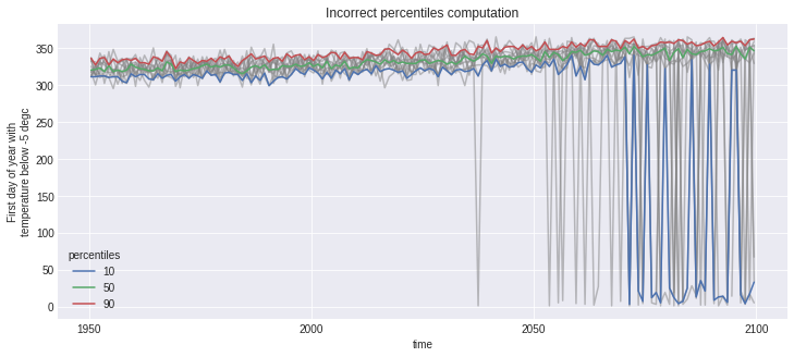
However, the first_day_below indicator is problematic. The data is in a “day of year” (doy) format, an integer starting at 1 on January 1st and going to 365 on December 31st (in our no leap calendar). There might be years where the first day below 0°C happened after December 31st, meaning that taking the percentiles directly will give incorrect results. The trick is simply to convert the “day of year” data to a format where the numerical order reflects the temporal order within each period.
The next graph show the incorrect version. Notice how for the years where some members have values in January (\(0 < doy \le 31\)), those “small” numerical values are classified into the 10th percentile, while they are in fact later dates, so should be considered so and classified as the 90th percentile.
out.first_day_below.plot(hue='realization', color='grey', alpha=0.5)
out_perc.first_day_below.plot(hue='percentiles')
plt.title('Incorrect percentiles computation');
# Convert "doys" to the number of days elapsed since the time coordinate (which is 1st of July)
fda_days_since = xclim.core.calendar.doy_to_days_since(out.first_day_below)

# Take percentiles now that the numerical ordering is correct
fda_days_since_perc = xclim.ensembles.ensemble_percentiles(fda_days_since, values=[10, 50, 90], split=False)

# Convert back to doys for meaningful values
fda_doy_perc = xclim.core.calendar.days_since_to_doy(fda_days_since_perc)

# Replace the bad data with the good one
out_perc['first_day_below'] = fda_doy_perc
Voilà! Lets enjoy our work!
with ProgressBar():
    out_perc.load()
[########################################] | 100% Completed | 20.9s
for name, var in out_perc.data_vars.items():
    plt.figure()
    var.plot(hue='percentiles')
    plt.title(name)
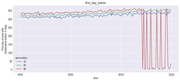
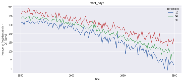
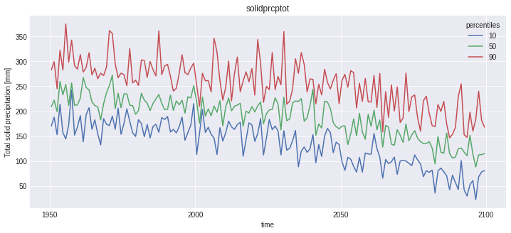
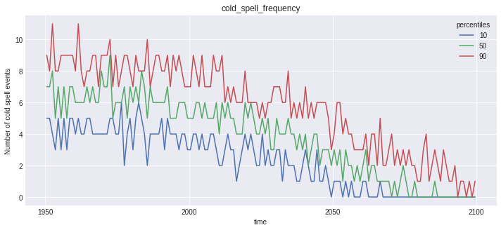
Notice that the doy conversion trick did work for first_day_below, but plotting this kind of variable is not straightforward, and not the point of this notebook.
Bias-adjustment
Besides climate indicators, xclim comes with the sdba (statistical downscaling and bias-adjustment) module. The module tries to follow a “modular” approach instead of implementing published methods as black box functions. It comes with some pre- and post-processing function in sdba.processing and a few adjustment objects in sdba.adjustment. Adjustment algorithms all conform to the train - adjust scheme, formalized within Adjustment classes. Given a reference time series (ref), historical simulations (hist) and simulations to be adjusted (sim), any bias-adjustment method would be applied by first estimating the adjustment factors between the historical simulation and the observations series, and then applying these factors to sim, which could be a future simulation.
Most algorithms implemented also perform the adjustment separately on temporal groups. For example, for a Quantile Mapping method, one would compute quantiles and adjustment factors for each day of the year individually or within a moving window, so that seasonal variations do not interfere with the result.
Simple quantile mapping
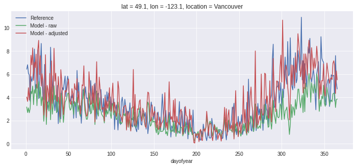
Let’s start here with a simple Empirical Quantile Mapping adjustment for pr. Instead of adjusting a future period, we adjust the historical timeseries, so we can have a clear appreciation of the adjustment results. This adjustment method is based on [1].
Multiplicative and Additive modes : In most of the literature, bias-adjustment involving pr is done in a multiplicative mode, in opposition to the additive mode used for temperatures. In xclim.sdba, this is controlled with the kind keyword, which defaults to '+' (additive). This means that sim values will be multiplied to the adjustment factors in the case kind='*', and added (or subtracted) with '+'.
# We are opening the datasets with xclim.testing.open_dataset
# a convenience function for accessing xclim's test and example datasets, stored in a github repository.
dsref = xclim.testing.open_dataset('sdba/ahccd_1950-2013.nc')
dssim = xclim.testing.open_dataset('sdba/CanESM2_1950-2100.nc')

# Extract 30 years of the daily data
# The data is made of 3 time series, we take only one "location"
# `ref` is given in Celsius, we must convert to Kelvin to fit with hist and sim
ref = dsref.pr.sel(time=slice('1980', '2010'), location='Vancouver')
ref = xclim.core.units.convert_units_to(ref, 'mm/d')
hist = dssim.pr.sel(time=slice('1980', '2010'), location='Vancouver')
hist = xclim.core.units.convert_units_to(hist, 'mm/d')

# We want to group data on a day-of-year basis with a 31-day moving window
group_doy_31 = xclim.sdba.Grouper('time.dayofyear', window=31)

# Create the adjustment object
EQM = xclim.sdba.EmpiricalQuantileMapping(nquantiles=15, group=group_doy_31, kind='*')

# Train it
EQM.train(ref, hist)

# Adjust hist
# And we estimate correct adjustment factors by interpolating linearly between quantiles
scen = EQM.adjust(hist, interp='linear')
# Plot the season cycle
fig, ax = plt.subplots()
ref.groupby('time.dayofyear').mean().plot(ax=ax, label='Reference')
hist.groupby('time.dayofyear').mean().plot(ax=ax, label='Model - raw')
scen.groupby('time.dayofyear').mean().plot(ax=ax, label='Model - adjusted')
ax.legend();
To inspect the trained adjustment data, we can access it with EQM.ds:
EQM.ds
<xarray.Dataset>
Dimensions:    (dayofyear: 365, quantiles: 17)
Coordinates:
  * quantiles  (quantiles) float64 1e-06 0.03333 0.1 0.1667 ... 0.9 0.9667 1.0
  * dayofyear  (dayofyear) int64 1 2 3 4 5 6 7 8 ... 359 360 361 362 363 364 365
Data variables:
    af         (dayofyear, quantiles) float64 nan 0.0 0.0 ... 1.377 1.684 1.686
    hist_q     (dayofyear, quantiles) float64 0.0 0.001463 ... 15.84 30.81
Attributes:
    _xclim_adjustment:  {"py/object": "xclim.sdba.adjustment.EmpiricalQuantil...
adj_params: EmpiricalQuantileMapping(nquantiles=15, kind='*', gro...- dayofyear: 365
- quantiles: 17
- quantiles(quantiles)float641e-06 0.03333 0.1 ... 0.9667 1.0
array([1.000000e-06, 3.333333e-02, 1.000000e-01, 1.666667e-01, 2.333333e-01, 3.000000e-01, 3.666667e-01, 4.333333e-01, 5.000000e-01, 5.666667e-01, 6.333333e-01, 7.000000e-01, 7.666667e-01, 8.333333e-01, 9.000000e-01, 9.666667e-01, 9.999990e-01]) - dayofyear(dayofyear)int641 2 3 4 5 6 ... 361 362 363 364 365
array([ 1, 2, 3, ..., 363, 364, 365])
- af(dayofyear, quantiles)float64nan 0.0 0.0 ... 1.377 1.684 1.686
- group :
- time.dayofyear
- group_compute_dims :
- ['time', 'window']
- group_window :
- 31
- kind :
- *
- standard_name :
- Adjustment factors
- long_name :
- Quantile mapping adjustment factors
array([[ nan, 0. , 0. , ..., 1.34326956, 1.6839163 , 1.68595758], [ nan, 0. , 0. , ..., 1.3399415 , 1.69931543, 1.87782013], [ nan, 0. , 0. , ..., 1.38112983, 1.80769705, 1.87790767], ..., [ nan, 0. , 0. , ..., 1.41380111, 1.64776177, 1.68613026], [ nan, 0. , 0. , ..., 1.39573133, 1.75821816, 1.68613019], [ nan, 0. , 0. , ..., 1.37734078, 1.6839163 , 1.68595758]]) - hist_q(dayofyear, quantiles)float640.0 0.001463 ... 15.84 30.81
- group :
- time.dayofyear
- group_compute_dims :
- ['time', 'window']
- group_window :
- 31
- standard_name :
- Model quantiles
- long_name :
- Quantiles of model on the reference period
array([[0.00000000e+00, 1.46299199e-03, 2.51842570e-02, ...,
        1.17176781e+01, 1.58410487e+01, 3.08093478e+01],
       [0.00000000e+00, 1.43809352e-03, 2.41532803e-02, ...,
        1.18512636e+01, 1.59236673e+01, 3.08093458e+01],
       [0.00000000e+00, 1.25626475e-03, 1.96289500e-02, ...,
        1.17657295e+01, 1.59213626e+01, 3.08093437e+01],
       ...,
       [0.00000000e+00, 1.65549644e-03, 2.70511758e-02, ...,
        1.10475227e+01, 1.56050070e+01, 3.08091608e+01],
       [0.00000000e+00, 1.46448681e-03, 2.41532803e-02, ...,
        1.13488892e+01, 1.58387625e+01, 3.08091631e+01],
       [0.00000000e+00, 1.43791665e-03, 2.22453354e-02, ...,
        1.15004220e+01, 1.58410487e+01, 3.08093478e+01]])
- _xclim_adjustment :
- {"py/object": "xclim.sdba.adjustment.EmpiricalQuantileMapping", "py/state": {"nquantiles": 15, "kind": "*", "group": {"py/object": "xclim.sdba.base.Grouper", "py/state": {"dim": "time", "add_dims": ["window"], "prop": "dayofyear", "name": "time.dayofyear", "window": 31, "interp": false}}, "hist_calendar": "noleap"}}
- adj_params :
- EmpiricalQuantileMapping(nquantiles=15, kind='*', group=Grouper(add_dims=['window'], name='time.dayofyear', window=31, interp=False))
More complex adjustment workflows can be created using the multiple tools exposed by xclim in sdba.processing and sdba.detrending. A more complete description of those is a bit too complex for the purposes of this notebook, but we invite interested users to look at the documentation.
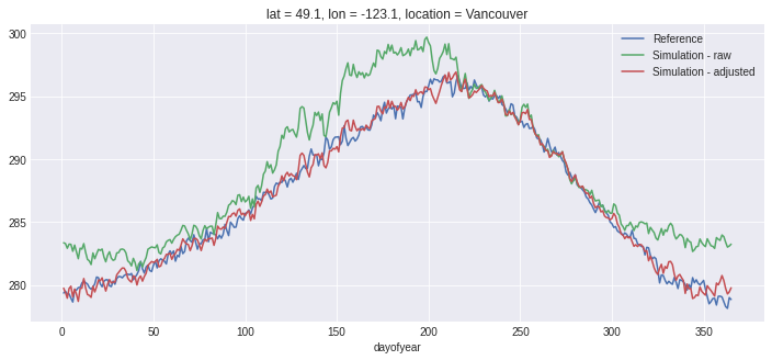
Let’s make another simple example, using the DetrendedQuantileMapping method. Compared to the EmpiricalQuantileMapping method, this one will normalize and detrend the inputs before computing the adjustment factors. This ensures a better quantile-to-quantile comparison when the climate change signal is strong. In reality, the same steps could all be performed explicitly, making use of xclim’s modularity, as is shown in the doc examples. It is based on [2].
# Extract the data.
ref = xclim.core.units.convert_units_to(
    dsref.tasmax.sel(time=slice('1980', '2010'), location='Vancouver'),
    'K'
)
hist = xclim.core.units.convert_units_to(
    dssim.tasmax.sel(time=slice('1980', '2010'), location='Vancouver'),
    'K'
)
sim = xclim.core.units.convert_units_to(
    dssim.tasmax.sel(location='Vancouver'),
    'K'
)


# Adjustment
DQM = xclim.sdba.DetrendedQuantileMapping(nquantiles=15, group=group_doy_31, kind='+')
DQM.train(ref, hist)

scen = DQM.adjust(sim, interp='linear', detrend=1)
fig, ax = plt.subplots()
ref.groupby('time.dayofyear').mean().plot(ax=ax, label='Reference'),
hist.groupby('time.dayofyear').mean().plot(ax=ax, label='Simulation - raw')
scen.sel(time=slice('1981', '2010')).groupby('time.dayofyear').mean().plot(ax=ax, label='Simulation - adjusted')
ax.legend();
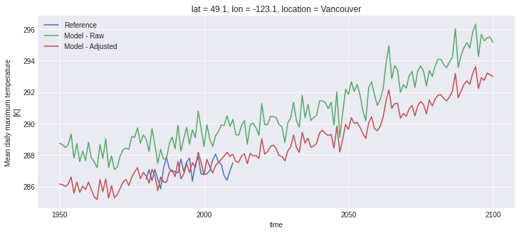
Just for fun, let’s compute the annual mean of the daily maximum temperature and plot the three time series:
with xclim.set_options(cf_compliance='log'):
    ref_tg = xclim.indicators.atmos.tx_mean(tasmax=ref)
    sim_tg = xclim.indicators.atmos.tx_mean(tasmax=sim)
    scen_tg = xclim.indicators.atmos.tx_mean(tasmax=scen)

fig, ax = plt.subplots()
ref_tg.plot(ax=ax, label='Reference')
sim_tg.plot(ax=ax, label='Model - Raw')
scen_tg.plot(ax=ax, label='Model - Adjusted')
ax.legend();
Finch : xclim as a service
This final part of the notebook demonstrates the use of finch to compute indicators over the web using the Web Processing Service (WPS) standard. When running this notebook on binder, a local server instance of finch is already running on port 5000. We will interact with it using birdy a lightweight WPS client built upon OWSLib.
What is a WPS?
Standardized by the OGC, WPS is a standard describing web requests and responses to and from geospatial processing services. The standard defines how process execution can be requested, and how the output from that process is handled. finch provides such a service, bundling xclim’s indicator and some other tools into individual processes.
It’s possible with WPS to either embed input data in the request, or pass a link to the data. In the latter case, the server will download data locally before performing its calculations. It’s also possible to use DAP links so the web server only streams the data it actually needs. In the following example, we use a subset of the ERA5 reanalysis data, available on xclim’s testdata GitHub repository.
from birdy import WPSClient

wps = WPSClient('http://localhost:5000')
dataurl = 'https://github.com/Ouranosinc/xclim-testdata/raw/main/ERA5/daily_surface_cancities_1990-1993.nc'
# As in xclim, processes and their inputs are documented
# by parsing the indicator's attributes:
help(wps.growing_degree_days)
Help on method growing_degree_days in module birdy.client.base:

growing_degree_days(tas=None, check_missing='any', cf_compliance='warn', data_validation='raise', thresh='4.0 degC', freq='YS', missing_options=None, variable=None, output_formats=None) method of birdy.client.base.WPSClient instance
    The sum of degree-days over the threshold temperature.

    Parameters
    ----------
    tas : ComplexData:mimetype:`application/x-netcdf`, :mimetype:`application/x-ogc-dods`
        NetCDF Files or archive (tar/zip) containing netCDF files.
    thresh : string
        Threshold temperature on which to base evaluation.
    freq : {'YS', 'MS', 'QS-DEC', 'AS-JUL'}string
        Resampling frequency.
    check_missing : {'any', 'wmo', 'pct', 'at_least_n', 'skip', 'from_context'}string
        Method used to determine which aggregations should be considered missing.
    missing_options : ComplexData:mimetype:`application/json`
        JSON representation of dictionary of missing method parameters.
    cf_compliance : {'log', 'warn', 'raise'}string
        Whether to log, warn or raise when inputs have non-CF-compliant attributes.
    data_validation : {'log', 'warn', 'raise'}string
        Whether to log, warn or raise when inputs fail data validation checks.
    variable : string
        Name of the variable in the NetCDF file.

    Returns
    -------
    output_netcdf : ComplexData:mimetype:`application/x-netcdf`
        The indicator values computed on the original input grid.
    output_log : ComplexData:mimetype:`text/plain`
        Collected logs during process run.
    ref : ComplexData:mimetype:`application/metalink+xml; version=4.0`
        Metalink file storing all references to output files.
# Through birdy, the indicator call looks a lot like the one from xclim
# but passing an url instead of an xarray object.
# Also, the `variable` argument tells which variable from the dataset to use.
response = wps.growing_degree_days(
    dataurl,
    thresh='5 degC',
    freq='MS',
    variable='tas'
)

response.get()
growing_degree_daysResponse(
    output_netcdf='http://localhost:5000/outputs/c3603da3-c7d7-11eb-8e02-8cec4b2c9db7/out.nc',
    output_log='http://localhost:5000/outputs/c3603da3-c7d7-11eb-8e02-8cec4b2c9db7/log.txt',
    ref='http://localhost:5000/outputs/c3603da3-c7d7-11eb-8e02-8cec4b2c9db7/input.meta4'
)
The response we received is a list of URLs pointing to output files. Birdy makes it easy to open links to datasets directly in xarray:
out = response.get(asobj=True).output_netcdf
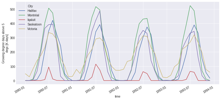
out.growing_degree_days.plot(hue='location');
Chain computations
As the goal of finch is to free the user of most, if not all, computation needs, it includes many other processes for all common climate analysis tasks. For example, here we will take maps of tasmax and tasmin over southern Québec, subset them with a square bounding box of lon/lat, compute tas as the mean of the other two and then finally, compute the growing season length with custom parameters.
All processes will be fed with the output of the previous one, so that no intermediate result is ever downloaded to the client. Only the last output is directly downloaded to file using python’s urllib.
tasmax_url = "https://github.com/Ouranosinc/xclim-testdata/raw/main/NRCANdaily/nrcan_canada_daily_tasmax_1990.nc"
tasmin_url = "https://github.com/Ouranosinc/xclim-testdata/raw/main/NRCANdaily/nrcan_canada_daily_tasmin_1990.nc"
pr_url = "https://github.com/Ouranosinc/xclim-testdata/raw/main/NRCANdaily/nrcan_canada_daily_pr_1990.nc"

# Subset the maps
resp_tx = wps.subset_bbox(tasmax_url, lon0=-72, lon1=-68, lat0=46, lat1=50)
resp_tn = wps.subset_bbox(tasmin_url, lon0=-72, lon1=-68, lat0=46, lat1=50)
resp_pr = wps.subset_bbox(pr_url, lon0=-72, lon1=-68, lat0=46, lat1=50)

# Compute tas
# We don't need to provide variable names because variables have the same names as the argument names
resp_tg = wps.tg(tasmin=resp_tn.get().output, tasmax=resp_tx.get().output)

# Compute growing season length, as defined by the period between
# Start/End when tas is over/under 10°C for 6 consecutive days
resp_lpr = wps.liquid_precip_ratio(
    pr=resp_pr.get().output,
    tas=resp_tg.get().output_netcdf,
    freq='YS'
)
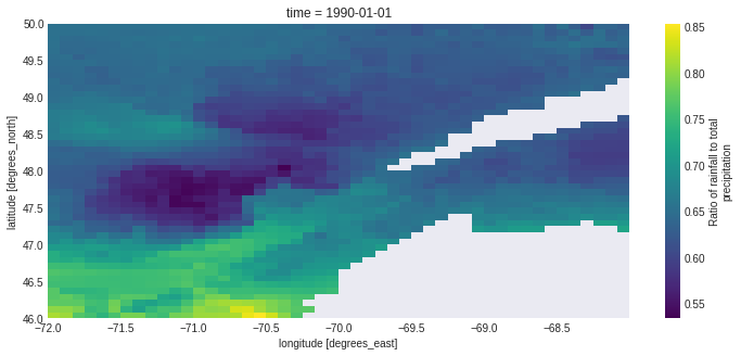
# Plot the liquid precipitation ratio of 1990
out_lpr = resp_lpr.get(asobj=True).output_netcdf
out_lpr.liquid_precip_ratio.plot()
<matplotlib.collections.QuadMesh at 0x7f0194f86700>
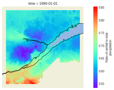
# or we can plot it as a map!
import cartopy.crs as ccrs
import cartopy.feature as cfeature

# Set a CRS transformation:
crs = ccrs.PlateCarree()

# Add some map elements
ax = plt.subplot(projection=crs)
ax.add_feature(cfeature.LAND)
ax.add_feature(cfeature.OCEAN)
ax.add_feature(cfeature.COASTLINE)
out_lpr.liquid_precip_ratio.plot(ax=ax, transform=crs, cmap="rainbow")

plt.show()
Output attributes are formatted the same as when xclim is used locally:
out_lpr.liquid_precip_ratio
<xarray.DataArray 'liquid_precip_ratio' (time: 1, lat: 48, lon: 48)>
array([[[0.65363 , 0.651616, ..., 0.63733 , 0.629445],
        [0.651229, 0.650147, ..., 0.629233, 0.636435],
        ...,
        [0.798548, 0.797585, ...,      nan,      nan],
        [0.812997, 0.806936, ...,      nan,      nan]]], dtype=float32)
Coordinates:
  * time     (time) datetime64[ns] 1990-01-01
  * lat      (lat) float32 49.96 49.88 49.79 49.71 ... 46.29 46.21 46.12 46.04
  * lon      (lon) float32 -71.96 -71.88 -71.79 -71.71 ... -68.21 -68.12 -68.04
Attributes:
    units:
    cell_methods:   tas: tasmin: time: minimum within days tasmax: time: maxi...
    xclim_history:  pr: \ntas: \n[2021-06-07 17:32:05] liquid_precip_ratio: L...
    long_name:      Ratio of rainfall to total precipitation
description: Annual ratio of rainfall to total precipitation. rainfall...- time: 1
- lat: 48
- lon: 48
- 0.6536 0.6516 0.652 0.6528 0.6519 0.6517 ... nan nan nan nan nan nan
array([[[0.65363 , 0.651616, ..., 0.63733 , 0.629445], [0.651229, 0.650147, ..., 0.629233, 0.636435], ..., [0.798548, 0.797585, ..., nan, nan], [0.812997, 0.806936, ..., nan, nan]]], dtype=float32) - time(time)datetime64[ns]1990-01-01
array(['1990-01-01T00:00:00.000000000'], dtype='datetime64[ns]')
- lat(lat)float3249.96 49.88 49.79 ... 46.12 46.04
- axis :
- Y
- units :
- degrees_north
- long_name :
- latitude
- standard_name :
- latitude
array([49.958332, 49.875 , 49.791668, 49.708332, 49.625 , 49.541668, 49.458332, 49.375 , 49.291668, 49.208332, 49.125 , 49.041668, 48.958332, 48.875 , 48.791668, 48.708332, 48.625 , 48.541668, 48.458332, 48.375 , 48.291668, 48.208332, 48.125 , 48.041668, 47.958332, 47.875 , 47.791668, 47.708332, 47.625 , 47.541668, 47.458332, 47.375 , 47.291668, 47.208332, 47.125 , 47.041668, 46.958332, 46.875 , 46.791668, 46.708332, 46.625 , 46.541668, 46.458332, 46.375 , 46.291668, 46.208332, 46.125 , 46.041668], dtype=float32) - lon(lon)float32-71.96 -71.88 ... -68.12 -68.04
- axis :
- X
- units :
- degrees_east
- long_name :
- longitude
- standard_name :
- longitude
array([-71.958336, -71.875   , -71.79167 , -71.708336, -71.625   , -71.54167 ,
       -71.458336, -71.375   , -71.29167 , -71.208336, -71.125   , -71.04167 ,
       -70.958336, -70.875   , -70.79167 , -70.708336, -70.625   , -70.54167 ,
       -70.458336, -70.375   , -70.29167 , -70.208336, -70.125   , -70.04167 ,
       -69.958336, -69.875   , -69.79167 , -69.708336, -69.625   , -69.54167 ,
       -69.458336, -69.375   , -69.29167 , -69.208336, -69.125   , -69.04167 ,
       -68.958336, -68.875   , -68.79167 , -68.708336, -68.625   , -68.54167 ,
       -68.458336, -68.375   , -68.29167 , -68.208336, -68.125   , -68.04167 ],
      dtype=float32)
- units :
- cell_methods :
- tas: tasmin: time: minimum within days tasmax: time: maximum within days time: mean within days
- xclim_history :
- pr: tas: [2021-06-07 17:32:05] liquid_precip_ratio: LIQUID_PRECIP_RATIO(pr=<array>, tas=<array>, thresh='0 degC', freq='YS', prsn=<class 'NoneType'>) - xclim version: 0.26.0.
- long_name :
- Ratio of rainfall to total precipitation
- description :
- Annual ratio of rainfall to total precipitation. rainfall is estimated as precipitation on days where temperature is above 0 degc.
Ensemble statistics
In addition to the indicators and the subsetting processes, finch wraps xclim’s ensemble statistics functionality in all-in-one processes. All indicator are provided in several ensemble-subset processes, where the inputs are subsetted before the indicator is computed and ensemble statistics taken. For example, ensemble_gridpoint_growing_season_length, which computes growing_season_length over a single gridpoint for all members of the specified ensemble. However, at least for the current version, ensemble datasets are hardcoded in the configuration of the server instance and one can’t send their own list of members.
In order not to overload Ouranos’ servers where these current hardcoded datasets are stored, no example of this is run by default here. But interested users are invited to uncomment the following lines to see for themselves.
The ensemble data used by this example is a bias-adjusted and downscaled product from the Pacific Climate Impacts Consortium (PCIC). It is described here.
help(wps.ensemble_grid_point_max_n_day_precipitation_amount)
Help on method ensemble_grid_point_max_n_day_precipitation_amount in module birdy.client.base:

ensemble_grid_point_max_n_day_precipitation_amount(lat, lon, rcp, check_missing='any', cf_compliance='warn', data_validation='raise', start_date=None, end_date=None, ensemble_percentiles='10,50,90', dataset_name=None, models='24MODELS', window=1, freq='YS', missing_options=None, output_format='netcdf', output_formats=None) method of birdy.client.base.WPSClient instance
    Calculate the n-day rolling sum of the original daily total precipitation series and determine the maximum value over each period.

    Parameters
    ----------
    lat : string
        Latitude coordinate. Accepts a comma separated list of floats for multiple grid cells.
    lon : string
        Longitude coordinate. Accepts a comma separated list of floats for multiple grid cells.
    start_date : string
        Initial date for temporal subsetting. Can be expressed as year (%Y), year-month (%Y-%m) or year-month-day(%Y-%m-%d). Defaults to first day in file.
    end_date : string
        Final date for temporal subsetting. Can be expressed as year (%Y), year-month (%Y-%m) or year-month-day(%Y-%m-%d). Defaults to last day in file.
    ensemble_percentiles : string
        Ensemble percentiles to calculate for input climate simulations. Accepts a comma separated list of integers.
    dataset_name : {'bccaqv2'}string
        Name of the dataset from which to get netcdf files for inputs.
    rcp : {'rcp26', 'rcp45', 'rcp85'}string
        Representative Concentration Pathway (RCP)
    models : {'24MODELS', 'PCIC12', 'BNU-ESM', 'CCSM4', 'CESM1-CAM5', 'CNRM-CM5', 'CSIRO-Mk3-6-0', 'CanESM2', 'FGOALS-g2', 'GFDL-CM3', ...}string
        When calculating the ensemble, include only these models. By default, all 24 models are used.
    window : integer
        Window size in days.
    freq : {'YS', 'MS', 'QS-DEC', 'AS-JUL'}string
        Resampling frequency.
    check_missing : {'any', 'wmo', 'pct', 'at_least_n', 'skip', 'from_context'}string
        Method used to determine which aggregations should be considered missing.
    missing_options : ComplexData:mimetype:`application/json`
        JSON representation of dictionary of missing method parameters.
    cf_compliance : {'log', 'warn', 'raise'}string
        Whether to log, warn or raise when inputs have non-CF-compliant attributes.
    data_validation : {'log', 'warn', 'raise'}string
        Whether to log, warn or raise when inputs fail data validation checks.
    output_format : {'netcdf', 'csv'}string
        Choose in which format you want to recieve the result

    Returns
    -------
    output : ComplexData:mimetype:`application/x-netcdf`, :mimetype:`application/zip`
        The format depends on the 'output_format' input parameter.
    output_log : ComplexData:mimetype:`text/plain`
        Collected logs during process run.
## Get maximal 5 days precipitation amount for Niagara Falls between 2040 and 2070
## for 12 rcp45 datasets bias-adjusted and downscaled with BCCAQv2 by PCIC
## Careful : this call will take a long time to succeed!

#resp_ens = wps.ensemble_grid_point_max_n_day_precipitation_amount(
#    lat=43.08,
#    lon=-79.07,
#    start_date='2040-01-01',
#    end_date='2070-12-31',
#    ensemble_percentiles=[10, 50, 90],
#    rcp='rcp45',
#    models='PCIC12',
#    window=5,
#    freq='YS',
#    data_validation='warn',
#)
#resp_ens.get(asobj=True).output
This concludes our xclim and finch tour! We hope these tools can be useful for your workflows. The development of both is always on-going, visit us at our GitHub pages for any questions or if you want to contribute!
References
Bias-adjustment
[1] Dequé, M. (2007). Frequency of precipitation and temperature extremes over France in an anthropogenic scenario: Model results and statistical correction according to observed values. Global and Planetary Change, 57(1–2), 16–26. https://doi.org/10.1016/j.gloplacha.2006.11.030
[2] Cannon, A. J., Sobie, S. R., & Murdock, T. Q. (2015). Bias correction of GCM precipitation by quantile mapping: How well do methods preserve changes in quantiles and extremes? Journal of Climate, 28(17), 6938–6959. https://doi.org/10.1175/JCLI-D-14-00754.1
Software used
xarray 0.18.2 : Stephan Hoyer, Joe Hamman, Maximilian Roos, keewis, Deepak Cherian, Clark Fitzgerald, … Benoit Bovy. (2021, May 19). pydata/xarray: v0.18.2 (Version v0.18.2). Zenodo. http://doi.org/10.5281/zenodo.4774304
numpy : Harris, C.R., Millman, K.J., van der Walt, S.J. et al. Array programming with NumPy. Nature 585, 357–362 (2020). DOI: 0.1038/s41586-020-2649-2
dask : Dask Development Team (2016). Dask: Library for dynamic task scheduling URL https://dask.org
cftime 1.4 : Jeff Whitaker, Constantine Khrulev, Spencer Clark, Joe Hamman, Bill Little, Ryan May, … Stefan. (2021, January 31). Unidata/cftime: version 1.4.0 release (Version v1.4.0rel). Zenodo. http://doi.org/10.5281/zenodo.4484141