Leveraging satellite data and pangeo to investigate the role of Gulf Stream frontal dynamics in ocean productivity
Authors
Author1 = {“name”: “Patrick Clifton Gray”, “affiliation”: “Duke University Marine Lab”, “email”: “patrick.c.gray@duke.edu”, “orcid”: “0000-0002-8997-5255”}
Author2 = {“name”: “David W. Johnston”, “affiliation”: “Duke University Marine Lab”, “email”: “david.johnston@duke.edu”, “orcid”: “0000-0003-2424-036X”}
Table of Contents
In a vessel floating on the Gulf Stream one sees nothing of the current and knows nothing but what experience tells him; but to be anchored in its depths far out of the sight of land, and to see the mighty torrent rushing past at a speed of miles per hour, day after day and day after day, one begins to think that all the wonders of the earth combined can not equal this one river in the ocean.” - J. E. Pillsbury, The Gulf Stream (1891)
Purpose
The Gulf Stream is a dominant physical feature in the North Atlantic, influencing the marine ecosystem across trophic levels, yet the physical-biological interactions along this western boundary current are poorly understood. In this work we analyze Gulf Stream physical and biological patterns over multiple years with particular emphasis on how the current’s front impacts biology across space and time. We ask specifically how phytoplankton patterns along the front correspond to seasonality and wind with speculation on possible nutrient limitations. This work primarily uses satellite-based sea surface temperature (SST), chlorophyll-a (chla), and sea surface height (SSH) data. Using xarray and running in jupyter in the cloud allows efficient analysis across many years of satellite data and holoviz enables interactive visualization and data exploration. Basing this work on a pangeo Docker image allows easy reproducibility and a robust set of packages for scientific computing. This work aims to provide insight into the overall role of Gulf Stream frontal features and dynamics in ocean productivity and increase the ease of access, manipulation, and visualization of these highly dimensional and complex datasets.
Technical contributions
collation and visualization of a variety of oceanographic datasets permitting investigation of the Gulf Stream front
derivation of the Gulf Stream front location every month for a decade from Sea Surface Height data
demonstration of an array of scientific computing tools for oceanography analysis
investigation of the physical and biological properties of the Gulf Stream front over a decade
Methodology
The goal of this analysis is to investigate the physical and biological trends and relationships along the Gulf Stream front using SST, wind, and chla data. For comparison we also investigate that same data on the coastal and open ocean side of the front. The first half of the notebook pulls in and visualizes all the different datasets and then derives the front location based on the 0.25m isoline in sea surface height data. The final step in the first half of the notebook is to select data from the main datasets (SST, wind, chla) using these front lines at every time step.
The second half of the notebook then analyzes this along-front data using a variety of visualizations and interprets the results.
Results
Results are discussed in detail throughout the analysis section. Some main takeaways are that for nearly all of the Gulf Stream, from Florida out into the North Atlantic, there is a fall bloom that is comparable or greater than the spring bloom and this is true on both sides of the front.
The northern region (further downstream) has a major increase in chla in the spring - the well studied spring bloom - and the region further south (upstream) around the South Atlantic Bight (SAB) has a relatively large increase throughout the whole winter, starting mid fall and staying high until the spring. The region around Cape Hatteras falls in the middle of these two patterns, but with generally higher chla, particularly on the coastal side, likely due to proximity to the coast and generally large outflows from Pamlico Sound and Chesapeake Bay injecting nutrients into the water. The sustained spikes in chla off Cape Hatteras near the front on the coastal side are likely drivers of the increased biodiversity in that region. It is also worth noting that the northerly section of the front (downstream) has a more notable mid-winter decrease, possibly when light begins to be limiting, and this is not as pronounced in the southerly section of the front (upstream). Though the light difference is not extreme. There are 9.5 hours of sunlight on the winter solstice at 37° N and 10.6 hours at 27° N.
The satellite imagery makes it clear that the Gulf Stream is a major boundary between the coastal and the open ocean ecosystems. A large increase in chla beyond the Gulf Stream front, in the Sargasso Sea, is evident from late fall to early spring. The spring bloom in the North Atlantic is also clear where it peaks in April and May.
The SST data matches what one might expect, decreasing throughout the winter and increasing in summer with the Gulf Stream itself staying as the warmest water throughout all seasons. We can also see a few eddy footprints in SST and SSH even though this data is resampled to monthly time steps.
Overall the analysis generally agrees with the understanding of phytoplankton dynamics in the Atlantic (Siegel et al 2002, Fischer et al 2015) but it doesn’t follow exactly along with the commonly studied bloom in the North Atlantic. Fall production is more intense along the Gulf Stream compared to the North Atlantic, potentially supplied with nutrients from mesoscale upwelling (Pascual et al 2014) and ageostrophic circulation at the front (Levy et al 2018) and supplied with seed populations from further south. This is more in agreement with ideas of winter biomass accumulation despite low light conditions (e.g. Boss and Behrenfeld 2010). Wind patterns are noisy and don’t lead to clear agreement or disagreement with the general assumptions that winter winds drive deeper mixing which inject nutrients supplying the bloom and stronger winds in the spring deepen mixed layers which delay the start of the subpolar spring (Ueyama and Monger 2005, Henson et al 2009), but this is an avenue for further investigation with additional wind datasets.
Funding
Award1 = {“agency”: “US National Aeronautics and Space Administration”, “award_code”: “80NSSC19K1366”, “award_URL”: “https://nspires.nasaprs.com/external/viewrepositorydocument/cmdocumentid=701992/solicitationId={913A7DEE-2747-6539-130C-0AB1E2322F42}/viewSolicitationDocument=1/Updated ESD FINESST19 SELECTIONS 7.24.19.pdf”}
Keywords
keywords=[“gulf stream”, “satellite oceanography”, “xarray”, “physical-biological”, “ocean productivity”]
Citation
Gray, P.C., & Johnston D.W., 2021. Leveraging satellite data and pangeo to investigate the role of Gulf Stream frontal dynamics in ocean productivity. Accessed 5/15/2021 at https://github.com/patrickcgray/gulf_stream_productivity_dynamics
Acknowledgements
We acknowledge helpful conversations with many collaborators and mentors as well as the substantial effort of the open source community developing xarray, zarr, holoviz, geopandas, jupyter and the many other libraries we relied on for this analysis.
Setup
Library import
# Data manipulation
import pandas as pd
import geopandas as gpd
import numpy as np
import xarray as xr
# time
import datetime
# downloading data from GDrive
from google_drive_downloader import GoogleDriveDownloader as gdd
# Options for pandas
pd.options.display.max_columns = 50
pd.options.display.max_rows = 30
# Visualizations
import hvplot.xarray
import hvplot.pandas
import matplotlib.pyplot as plt
from matplotlib.colors import LogNorm
# geographic and geometry tools
import cartopy.crs as crs
from shapely.ops import unary_union
from shapely.ops import transform
from shapely.geometry import Polygon
from affine import Affine
# there are many divide by zero warnings that we're going to suppress
# but advised to comment this line out when actively coding
import warnings
warnings.filterwarnings('ignore')
Local library import
# this is a package from https://github.com/GeoscienceAustralia/dea-notebooks that allows contours to be pulled from xarray datasets via geopanda points
from dea_spatial import subpixel_contours
Data preparation
Data is all stored as zarr and downloaded from Google Drive in the next code block. This is done to ensure speed of operation for this notebook. Current data providers are too slow for use in an ephemeral Binder environment and some require manual downloading. All data can be downloaded from the original repositories via the information below if needed. All data use the same bounds, the latitude range is from 44° North to 26° North and the longitude range is from 82° West to 66° West.
Altimetry data
is from AVISO distributed via Copernicus and uses multiple altimeters to generate a 0.25 degree daily SSH and (sea level anomaly) SLA product. The data can be downloaded here. After navigating to that site the user must manually search for SEALEVEL_GLO_PHY_L4_NRT_OBSERVATIONS_008_046 and specify the bounds and time period (January 1st, 2010 through December 31st 2019).
Ocean Color data
is from the Ocean Colour Climate Change Initiative’s multi-sensor global satellite chlorophyll-a product we use the CCI_ALL-v5.0-8DAY product which can viewed here and our exact dataset can be downloaded with this link.
Sea Surface Temperature
is the GHRSST Level 4 OSPO Global Nighttime Foundation Sea Surface Temperature Analysis product. More can be found on this product here and all data can be downloaded here.
Wind speed data
is Metop-A ASCAT, 0.25°, Global, Near Real Time, 2009-present (8 Day) available for download here. And for this exact dataset this link can be used.
Data download
Download all the necessary files from Google Drive. This should take approximately 1-2 minutes to download the ~1GB of data,
file_ids = [
'1KVDlXdaqPCi_gomHn6QK76NYmF7RONT5',
'1MRUr0wAhVFIdrFjUg0YcDjaKaABKs09o',
'1gw7BG7wlZfU_BGNDf3QH1UARWUjwsIjz',
'1Cwl0gLUHFTwkvdSEm1KZiAsUU7jZyrAN'
]
paths = [
'aviso.zip',
'chla.zip',
'sst.zip',
'winds.zip'
]
for f, p in zip(file_ids, paths):
gdd.download_file_from_google_drive(file_id=f,
dest_path='./data/'+ p,
showsize=True,
unzip=True)
Downloading 1KVDlXdaqPCi_gomHn6QK76NYmF7RONT5 into ./data/aviso.zip...
65.0 MiB Done.
Unzipping...Done.
Downloading 1MRUr0wAhVFIdrFjUg0YcDjaKaABKs09o into ./data/chla.zip...
217.3 MiB Done.
Unzipping...Done.
Downloading 1gw7BG7wlZfU_BGNDf3QH1UARWUjwsIjz into ./data/sst.zip...
83.2 MiB Done.
Unzipping...Done.
Downloading 1Cwl0gLUHFTwkvdSEm1KZiAsUU7jZyrAN into ./data/winds.zip...
14.3 MiB Done.
Unzipping...Done.
Data import
Here we pull all data into the notebook from local storage and do some preliminary visualization and data prep.
The chlorophyll-a data, altimetry, and wind data cover 2010 through the end of 2019. The sea surface temp dataset covers 2017 through 2019.
Chlorophyll-a
from the Ocean Colour Climate Change Initiative project. This is 5 day averaged product generated by merging data from many sources including MODIS Aqua, Sentinel-3, MERIS and more.
chla_ds = xr.open_zarr('data/chla_long.zarr')
chla_ds
<xarray.Dataset>
Dimensions: (lat: 432, lon: 384, time: 714)
Coordinates:
* lat (lat) float64 43.98 43.94 43.9 43.85 ... 26.15 26.1 26.06 26.02
* lon (lon) float64 -81.98 -81.94 -81.9 -81.85 ... -66.1 -66.06 -66.02
* time (time) datetime64[ns] 2010-04-01 2010-04-06 ... 2019-12-27
Data variables:
chlor_a (time, lat, lon) float32 dask.array<chunksize=(238, 218, 320), meta=np.ndarray>
Attributes: (12/50)
Conventions: CF-1.7
Metadata_Conventions: Unidata Dataset Discovery v1.0
_NCProperties: version=1|netcdflibversion=4.4.1.1|hdf...
cdm_data_type: Grid
comment: See summary attribute
creation_date: Tue Feb 2 11:54:34 2021
... ...
time_coverage_duration: P5D
time_coverage_end: 202012302359Z
time_coverage_resolution: P5D
time_coverage_start: 202012260000Z
title: ESA CCI Ocean Colour Product
tracking_id: 2a3b7595-7123-4795-8013-71659996a2d8- lat: 432
- lon: 384
- time: 714
- lat(lat)float6443.98 43.94 43.9 ... 26.06 26.02
- _ChunkSizes :
- 270
- axis :
- Y
- long_name :
- latitude
- standard_name :
- latitude
- units :
- degrees_north
- valid_max :
- 89.97916666666667
- valid_min :
- -89.97916666666666
array([43.979167, 43.9375 , 43.895833, ..., 26.104167, 26.0625 , 26.020833])
- lon(lon)float64-81.98 -81.94 ... -66.06 -66.02
- _ChunkSizes :
- 270
- axis :
- X
- long_name :
- longitude
- standard_name :
- longitude
- units :
- degrees_east
- valid_max :
- 179.97916666666663
- valid_min :
- -179.97916666666666
array([-81.979167, -81.9375 , -81.895833, ..., -66.104167, -66.0625 , -66.020833]) - time(time)datetime64[ns]2010-04-01 ... 2019-12-27
- _ChunkSizes :
- 1
- axis :
- T
- standard_name :
- time
array(['2010-04-01T00:00:00.000000000', '2010-04-06T00:00:00.000000000', '2010-04-11T00:00:00.000000000', ..., '2019-12-17T00:00:00.000000000', '2019-12-22T00:00:00.000000000', '2019-12-27T00:00:00.000000000'], dtype='datetime64[ns]')
- chlor_a(time, lat, lon)float32dask.array<chunksize=(238, 218, 320), meta=np.ndarray>
- _ChunkSizes :
- [1, 270, 270]
- ancillary_variables :
- chlor_a_log10_rmsd chlor_a_log10_bias
- grid_mapping :
- crs
- long_name :
- Chlorophyll-a concentration in seawater (not log-transformed), generated by as a blended combination of OCI, OCI2, OC2 and OCx algorithms, depending on water class memberships
- parameter_vocab_uri :
- http://vocab.ndg.nerc.ac.uk/term/P011/current/CHLTVOLU
- standard_name :
- mass_concentration_of_chlorophyll_a_in_sea_water
- units :
- milligram m-3
- units_nonstandard :
- mg m^-3
Array Chunk Bytes 451.83 MiB 63.33 MiB Shape (714, 432, 384) (238, 218, 320) Count 13 Tasks 12 Chunks Type float32 numpy.ndarray
- Conventions :
- CF-1.7
- Metadata_Conventions :
- Unidata Dataset Discovery v1.0
- _NCProperties :
- version=1|netcdflibversion=4.4.1.1|hdf5libversion=1.8.20
- cdm_data_type :
- Grid
- comment :
- See summary attribute
- creation_date :
- Tue Feb 2 11:54:34 2021
- creator_email :
- help@esa-oceancolour-cci.org
- creator_name :
- Plymouth Marine Laboratory
- creator_url :
- http://esa-oceancolour-cci.org
- date_created :
- Tue Feb 2 11:54:34 2021
- geospatial_lat_max :
- 90.0
- geospatial_lat_min :
- -90.0
- geospatial_lat_resolution :
- .04166666666666666666
- geospatial_lat_units :
- decimal degrees north
- geospatial_lon_max :
- 180.0
- geospatial_lon_min :
- -180.0
- geospatial_lon_resolution :
- .04166666666666666666
- geospatial_lon_units :
- decimal degrees east
- geospatial_vertical_max :
- 0.0
- geospatial_vertical_min :
- 0.0
- git_commit_hash :
- 1898332e6ec0c2b15bdc7126194bbd777370800f
- history :
- Source data were: ESACCI-OC-L3S-OC_PRODUCTS-MERGED-1D_DAILY_4km_GEO_PML_OCx_QAA-20201226-fv5.0.nc, ESACCI-OC-L3S-OC_PRODUCTS-MERGED-1D_DAILY_4km_GEO_PML_OCx_QAA-20201227-fv5.0.nc, ESACCI-OC-L3S-OC_PRODUCTS-MERGED-1D_DAILY_4km_GEO_PML_OCx_QAA-20201228-fv5.0.nc, ESACCI-OC-L3S-OC_PRODUCTS-MERGED-1D_DAILY_4km_GEO_PML_OCx_QAA-20201229-fv5.0.nc, ESACCI-OC-L3S-OC_PRODUCTS-MERGED-1D_DAILY_4km_GEO_PML_OCx_QAA-20201230-fv5.0.nc; netcdf_compositor_cci composites Rrs_412, Rrs_443, Rrs_490, Rrs_510, Rrs_560, Rrs_665, water_class1, water_class2, water_class3, water_class4, water_class5, water_class6, water_class7, water_class8, water_class9, water_class10, water_class11, water_class12, water_class13, water_class14, atot_412, atot_443, atot_490, atot_510, atot_560, atot_665, aph_412, aph_443, aph_490, aph_510, aph_560, aph_665, adg_412, adg_443, adg_490, adg_510, adg_560, adg_665, bbp_412, bbp_443, bbp_490, bbp_510, bbp_560, bbp_665, chlor_a, kd_490, Rrs_412_bias, Rrs_443_bias, Rrs_490_bias, Rrs_510_bias, Rrs_560_bias, Rrs_665_bias, chlor_a_log10_bias, aph_412_bias, aph_443_bias, aph_490_bias, aph_510_bias, aph_560_bias, aph_665_bias, adg_412_bias, adg_443_bias, adg_490_bias, adg_510_bias, adg_560_bias, adg_665_bias, kd_490_bias with --mean, Rrs_412_rmsd, Rrs_443_rmsd, Rrs_490_rmsd, Rrs_510_rmsd, Rrs_560_rmsd, Rrs_665_rmsd, chlor_a_log10_rmsd, aph_412_rmsd, aph_443_rmsd, aph_490_rmsd, aph_510_rmsd, aph_560_rmsd, aph_665_rmsd, adg_412_rmsd, adg_443_rmsd, adg_490_rmsd, adg_510_rmsd, adg_560_rmsd, adg_665_rmsd, kd_490_rmsd with --root-mean-square, and MODISA_nobs, VIIRS_nobs, OLCI_nobs, MERIS_nobs, SeaWiFS_nobs, total_nobs - with --total
- id :
- ESACCI-OC-L3S-OC_PRODUCTS-MERGED-5D_DAILY_4km_GEO_PML_OCx_QAA-20201226-fv5.0.nc
- institution :
- Plymouth Marine Laboratory
- keywords :
- satellite,observation,ocean,ocean colour
- keywords_vocabulary :
- none
- license :
- ESA CCI Data Policy: free and open access. When referencing, please use: Ocean Colour Climate Change Initiative dataset, Version <Version Number>, European Space Agency, available online at http://www.esa-oceancolour-cci.org. We would also appreciate being notified of publications so that we can list them on the project website at http://www.esa-oceancolour-cci.org/?q=publications
- naming_authority :
- uk.ac.pml
- number_of_bands_used_to_classify :
- 4
- number_of_files_composited :
- 5
- number_of_optical_water_types :
- 14
- platform :
- Orbview-2,Aqua,Envisat,Suomi-NPP, Sentinel-3a
- processing_level :
- Level-3
- product_version :
- 5.0
- project :
- Climate Change Initiative - European Space Agency
- references :
- http://www.esa-oceancolour-cci.org/
- sensor :
- SeaWiFS,MODIS,MERIS,VIIRS,OLCI
- sensors_present :
- MODISA OLCIa VIIRSN
- source :
- NASA SeaWiFS L1A and L2 R2018.0 LAC and GAC, MODIS-Aqua L1A and L2 R2018.0, MERIS L1B 3rd reprocessing inc OCL corrections, NASA VIIRS L1A and L2 R2018.0, OLCI L1B
- spatial_resolution :
- 4km nominal at equator
- standard_name_vocabulary :
- NetCDF Climate and Forecast (CF) Metadata Conventions Version 1.7
- start_date :
- 26-DEC-2020 00:00:00.000000
- stop_date :
- 30-DEC-2020 23:59:00.000000
- summary :
- Data products generated by the Ocean Colour component of the European Space Agency Climate Change Initiative project. These files are 5 day composites of merged sensor (MERIS, MODIS Aqua, SeaWiFS LAC & GAC, VIIRS, OLCI) products. MODIS Aqua and SeaWiFS were band-shifted and bias-corrected to MERIS bands and values using a temporally and spatially varying scheme based on the overlap years of 2003-2007. VIIRS was band-shifted and bias-corrected in a second stage against the MODIS Rrs that had already been corrected to MERIS levels, for the overlap period 2012-2013; and at the third stage OLCI was bias corrected against already corrected MODIS, for overlap period 2016-07-01 to 2019-06-30. VIIRS, MODIS, SeaWiFS and MERIS Rrs were derived from a combination of NASA's l2gen (for basic sensor geometry corrections, etc) and HYGEOS Polymer v4.12 (for atmospheric correction). OLCI Rrs were sourced at L1b (already geometrically corrected) and processed with polymer. The Rrs were binned to a sinusoidal 4km level-3 grid, and later to 4km geographic projection, by Brockmann Consult's SNAP. Derived products were generally computed with the standard algorithmsthrough SeaDAS. QAA IOPs were derived using the standard SeaDAS algorithm but with a modified backscattering table to match that used in the bandshifting. The final chlorophyll is a combination of OCI, OCI2, OC2 and OCx, depending on the water class memberships. Uncertainty estimates were added using the fuzzy water classifier and uncertainty estimation algorithm of Tim Moore as documented in Jackson et al (2017). and updated accorsing to Jackson et al. (in prep).
- time_coverage_duration :
- P5D
- time_coverage_end :
- 202012302359Z
- time_coverage_resolution :
- P5D
- time_coverage_start :
- 202012260000Z
- title :
- ESA CCI Ocean Colour Product
- tracking_id :
- 2a3b7595-7123-4795-8013-71659996a2d8
Check out how the data is chunked and its dimensions.
chla_ds.chlor_a
<xarray.DataArray 'chlor_a' (time: 714, lat: 432, lon: 384)>
dask.array<open_dataset-f28549adf415f107edfc5d95f7debc63chlor_a, shape=(714, 432, 384), dtype=float32, chunksize=(238, 218, 320), chunktype=numpy.ndarray>
Coordinates:
* lat (lat) float64 43.98 43.94 43.9 43.85 ... 26.15 26.1 26.06 26.02
* lon (lon) float64 -81.98 -81.94 -81.9 -81.85 ... -66.1 -66.06 -66.02
* time (time) datetime64[ns] 2010-04-01 2010-04-06 ... 2019-12-27
Attributes:
_ChunkSizes: [1, 270, 270]
ancillary_variables: chlor_a_log10_rmsd chlor_a_log10_bias
grid_mapping: crs
long_name: Chlorophyll-a concentration in seawater (not log-tr...
parameter_vocab_uri: http://vocab.ndg.nerc.ac.uk/term/P011/current/CHLTVOLU
standard_name: mass_concentration_of_chlorophyll_a_in_sea_water
units: milligram m-3
units_nonstandard: mg m^-3- time: 714
- lat: 432
- lon: 384
- dask.array<chunksize=(238, 218, 320), meta=np.ndarray>
Array Chunk Bytes 451.83 MiB 63.33 MiB Shape (714, 432, 384) (238, 218, 320) Count 13 Tasks 12 Chunks Type float32 numpy.ndarray - lat(lat)float6443.98 43.94 43.9 ... 26.06 26.02
- _ChunkSizes :
- 270
- axis :
- Y
- long_name :
- latitude
- standard_name :
- latitude
- units :
- degrees_north
- valid_max :
- 89.97916666666667
- valid_min :
- -89.97916666666666
array([43.979167, 43.9375 , 43.895833, ..., 26.104167, 26.0625 , 26.020833])
- lon(lon)float64-81.98 -81.94 ... -66.06 -66.02
- _ChunkSizes :
- 270
- axis :
- X
- long_name :
- longitude
- standard_name :
- longitude
- units :
- degrees_east
- valid_max :
- 179.97916666666663
- valid_min :
- -179.97916666666666
array([-81.979167, -81.9375 , -81.895833, ..., -66.104167, -66.0625 , -66.020833]) - time(time)datetime64[ns]2010-04-01 ... 2019-12-27
- _ChunkSizes :
- 1
- axis :
- T
- standard_name :
- time
array(['2010-04-01T00:00:00.000000000', '2010-04-06T00:00:00.000000000', '2010-04-11T00:00:00.000000000', ..., '2019-12-17T00:00:00.000000000', '2019-12-22T00:00:00.000000000', '2019-12-27T00:00:00.000000000'], dtype='datetime64[ns]')
- _ChunkSizes :
- [1, 270, 270]
- ancillary_variables :
- chlor_a_log10_rmsd chlor_a_log10_bias
- grid_mapping :
- crs
- long_name :
- Chlorophyll-a concentration in seawater (not log-transformed), generated by as a blended combination of OCI, OCI2, OC2 and OCx algorithms, depending on water class memberships
- parameter_vocab_uri :
- http://vocab.ndg.nerc.ac.uk/term/P011/current/CHLTVOLU
- standard_name :
- mass_concentration_of_chlorophyll_a_in_sea_water
- units :
- milligram m-3
- units_nonstandard :
- mg m^-3
Visualize the first time step of the data
fig,ax = plt.subplots(figsize=(12,8))
chla_ds = chla_ds.sel(lat=slice(44,26),lon=slice(-82,-66))
chla_ds.chlor_a[0].plot(ax=ax, cmap='jet', norm=LogNorm(vmin=0.01, vmax=10))
<matplotlib.collections.QuadMesh at 0x7f5fc02ada00>
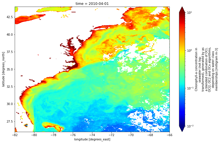
And now use hvplot to make the plotting interactive and add the ability to move through each time step with the scroll bar on the right.
proj = crs.Orthographic(-90, 30)
chla_ds.chlor_a.hvplot.quadmesh(
'lon', 'lat', projection=proj, project=True,
cmap='jet', dynamic=True, coastline='10m',
frame_width=300, logz=True, clim=(0.01,20), rasterize=True)
Sea Surface Height
via AVISO which uses multiple altimeters to generate a .25 degree daily SSH and SLA product.
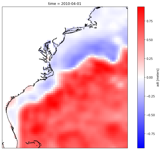
Note that the data variable we’re using in this xarray dataset is called adt which stands for absolute dynamic topography and is our SSH variable.
ssh_ds = xr.open_zarr('data/aviso.zarr')
ssh_ds
<xarray.Dataset>
Dimensions: (latitude: 72, longitude: 64, time: 713)
Coordinates:
* latitude (latitude) float32 26.12 26.38 26.62 26.88 ... 43.38 43.62 43.88
* longitude (longitude) float32 -81.88 -81.62 -81.38 ... -66.62 -66.38 -66.12
* time (time) datetime64[ns] 2010-04-01 2010-04-06 ... 2019-12-30
Data variables:
adt (time, latitude, longitude) float64 dask.array<chunksize=(179, 18, 32), meta=np.ndarray>
sla (time, latitude, longitude) float64 dask.array<chunksize=(179, 18, 32), meta=np.ndarray>
ugos (time, latitude, longitude) float64 dask.array<chunksize=(179, 18, 32), meta=np.ndarray>
vgos (time, latitude, longitude) float64 dask.array<chunksize=(179, 18, 32), meta=np.ndarray>- latitude: 72
- longitude: 64
- time: 713
- latitude(latitude)float3226.12 26.38 26.62 ... 43.62 43.88
- _ChunkSizes :
- 50
- _CoordinateAxisType :
- Lat
- axis :
- Y
- bounds :
- lat_bnds
- long_name :
- Latitude
- standard_name :
- latitude
- units :
- degrees_north
- valid_max :
- 89.875
- valid_min :
- -89.875
array([26.125, 26.375, 26.625, 26.875, 27.125, 27.375, 27.625, 27.875, 28.125, 28.375, 28.625, 28.875, 29.125, 29.375, 29.625, 29.875, 30.125, 30.375, 30.625, 30.875, 31.125, 31.375, 31.625, 31.875, 32.125, 32.375, 32.625, 32.875, 33.125, 33.375, 33.625, 33.875, 34.125, 34.375, 34.625, 34.875, 35.125, 35.375, 35.625, 35.875, 36.125, 36.375, 36.625, 36.875, 37.125, 37.375, 37.625, 37.875, 38.125, 38.375, 38.625, 38.875, 39.125, 39.375, 39.625, 39.875, 40.125, 40.375, 40.625, 40.875, 41.125, 41.375, 41.625, 41.875, 42.125, 42.375, 42.625, 42.875, 43.125, 43.375, 43.625, 43.875], dtype=float32) - longitude(longitude)float32-81.88 -81.62 ... -66.38 -66.12
array([-81.875, -81.625, -81.375, -81.125, -80.875, -80.625, -80.375, -80.125, -79.875, -79.625, -79.375, -79.125, -78.875, -78.625, -78.375, -78.125, -77.875, -77.625, -77.375, -77.125, -76.875, -76.625, -76.375, -76.125, -75.875, -75.625, -75.375, -75.125, -74.875, -74.625, -74.375, -74.125, -73.875, -73.625, -73.375, -73.125, -72.875, -72.625, -72.375, -72.125, -71.875, -71.625, -71.375, -71.125, -70.875, -70.625, -70.375, -70.125, -69.875, -69.625, -69.375, -69.125, -68.875, -68.625, -68.375, -68.125, -67.875, -67.625, -67.375, -67.125, -66.875, -66.625, -66.375, -66.125], dtype=float32) - time(time)datetime64[ns]2010-04-01 ... 2019-12-30
array(['2010-04-01T00:00:00.000000000', '2010-04-06T00:00:00.000000000', '2010-04-11T00:00:00.000000000', ..., '2019-12-20T00:00:00.000000000', '2019-12-25T00:00:00.000000000', '2019-12-30T00:00:00.000000000'], dtype='datetime64[ns]')
- adt(time, latitude, longitude)float64dask.array<chunksize=(179, 18, 32), meta=np.ndarray>
Array Chunk Bytes 25.07 MiB 805.50 kiB Shape (713, 72, 64) (179, 18, 32) Count 33 Tasks 32 Chunks Type float64 numpy.ndarray - sla(time, latitude, longitude)float64dask.array<chunksize=(179, 18, 32), meta=np.ndarray>
Array Chunk Bytes 25.07 MiB 805.50 kiB Shape (713, 72, 64) (179, 18, 32) Count 33 Tasks 32 Chunks Type float64 numpy.ndarray - ugos(time, latitude, longitude)float64dask.array<chunksize=(179, 18, 32), meta=np.ndarray>
Array Chunk Bytes 25.07 MiB 805.50 kiB Shape (713, 72, 64) (179, 18, 32) Count 33 Tasks 32 Chunks Type float64 numpy.ndarray - vgos(time, latitude, longitude)float64dask.array<chunksize=(179, 18, 32), meta=np.ndarray>
Array Chunk Bytes 25.07 MiB 805.50 kiB Shape (713, 72, 64) (179, 18, 32) Count 33 Tasks 32 Chunks Type float64 numpy.ndarray
Again inspect chunking and data details.
ssh_ds.adt
<xarray.DataArray 'adt' (time: 713, latitude: 72, longitude: 64)> dask.array<open_dataset-50a4e95be6b7da53cda52f698544c8d5adt, shape=(713, 72, 64), dtype=float64, chunksize=(179, 18, 32), chunktype=numpy.ndarray> Coordinates: * latitude (latitude) float32 26.12 26.38 26.62 26.88 ... 43.38 43.62 43.88 * longitude (longitude) float32 -81.88 -81.62 -81.38 ... -66.62 -66.38 -66.12 * time (time) datetime64[ns] 2010-04-01 2010-04-06 ... 2019-12-30
- time: 713
- latitude: 72
- longitude: 64
- dask.array<chunksize=(179, 18, 32), meta=np.ndarray>
Array Chunk Bytes 25.07 MiB 805.50 kiB Shape (713, 72, 64) (179, 18, 32) Count 33 Tasks 32 Chunks Type float64 numpy.ndarray - latitude(latitude)float3226.12 26.38 26.62 ... 43.62 43.88
- _ChunkSizes :
- 50
- _CoordinateAxisType :
- Lat
- axis :
- Y
- bounds :
- lat_bnds
- long_name :
- Latitude
- standard_name :
- latitude
- units :
- degrees_north
- valid_max :
- 89.875
- valid_min :
- -89.875
array([26.125, 26.375, 26.625, 26.875, 27.125, 27.375, 27.625, 27.875, 28.125, 28.375, 28.625, 28.875, 29.125, 29.375, 29.625, 29.875, 30.125, 30.375, 30.625, 30.875, 31.125, 31.375, 31.625, 31.875, 32.125, 32.375, 32.625, 32.875, 33.125, 33.375, 33.625, 33.875, 34.125, 34.375, 34.625, 34.875, 35.125, 35.375, 35.625, 35.875, 36.125, 36.375, 36.625, 36.875, 37.125, 37.375, 37.625, 37.875, 38.125, 38.375, 38.625, 38.875, 39.125, 39.375, 39.625, 39.875, 40.125, 40.375, 40.625, 40.875, 41.125, 41.375, 41.625, 41.875, 42.125, 42.375, 42.625, 42.875, 43.125, 43.375, 43.625, 43.875], dtype=float32) - longitude(longitude)float32-81.88 -81.62 ... -66.38 -66.12
array([-81.875, -81.625, -81.375, -81.125, -80.875, -80.625, -80.375, -80.125, -79.875, -79.625, -79.375, -79.125, -78.875, -78.625, -78.375, -78.125, -77.875, -77.625, -77.375, -77.125, -76.875, -76.625, -76.375, -76.125, -75.875, -75.625, -75.375, -75.125, -74.875, -74.625, -74.375, -74.125, -73.875, -73.625, -73.375, -73.125, -72.875, -72.625, -72.375, -72.125, -71.875, -71.625, -71.375, -71.125, -70.875, -70.625, -70.375, -70.125, -69.875, -69.625, -69.375, -69.125, -68.875, -68.625, -68.375, -68.125, -67.875, -67.625, -67.375, -67.125, -66.875, -66.625, -66.375, -66.125], dtype=float32) - time(time)datetime64[ns]2010-04-01 ... 2019-12-30
array(['2010-04-01T00:00:00.000000000', '2010-04-06T00:00:00.000000000', '2010-04-11T00:00:00.000000000', ..., '2019-12-20T00:00:00.000000000', '2019-12-25T00:00:00.000000000', '2019-12-30T00:00:00.000000000'], dtype='datetime64[ns]')
Let’s add on the attribute these units are meters
ssh_ds.adt.attrs["units"] = 'meters'
Visualize one time step of the absolute dynamic topography (ADT) variable in this dataset.
fig, ax = plt.subplots(figsize=(12,9), subplot_kw=dict(projection=crs.PlateCarree()))
ssh_ds.adt[0].plot(ax=ax, cmap='bwr')
ax.coastlines(resolution='10m')
ax.set_ylim(26,44)
ax.set_xlim(-82,-66)
(-82.0, -66.0)
Now use hvplot to allow interactive visualization of this dataset
proj = crs.Orthographic(-90, 30)
ssh_ds.adt.hvplot.quadmesh(
'longitude', 'latitude', projection=proj, project=True,
cmap='bwr', dynamic=True, coastline='10m',
frame_width=300, clim=(-1,1), rasterize=True)
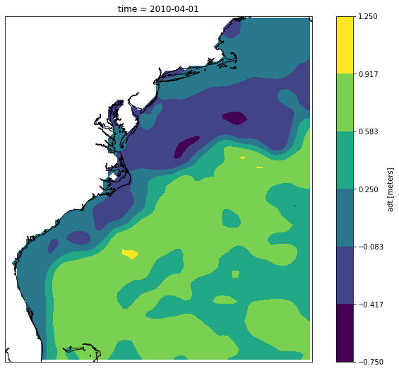
We’ll be using contours below (aka isolines in the sea surface height) to determine the location of the Gulf Stream front so let’s see what that looks like now
fig, ax = plt.subplots(figsize=(12,9), subplot_kw=dict(projection=crs.PlateCarree()))
ssh_ds.adt[0].plot.contourf(ax=ax, vmin=-1,vmax=1,center=0.25)
ax.coastlines(resolution='10m')
ax.set_ylim(26,44)
ax.set_xlim(-82,-66)
(-82.0, -66.0)
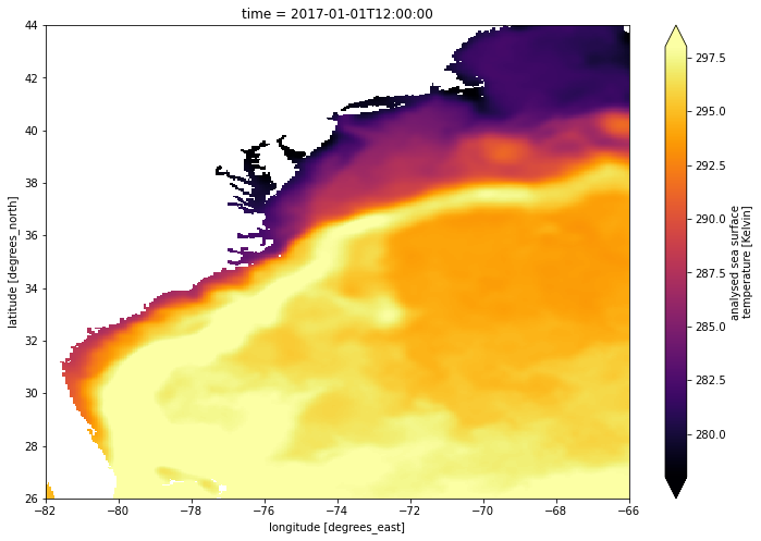
Sea Surface Temperature
via NOAA and the Group for High Resolution Sea Surface Temperature (GHRSST).
sst_ds = xr.open_zarr('data/sst.zarr')
sst_ds
<xarray.Dataset>
Dimensions: (lat: 360, lon: 320, time: 1089)
Coordinates:
* lat (lat) float32 26.02 26.08 26.12 26.17 ... 43.88 43.92 43.97
* lon (lon) float32 -81.97 -81.93 -81.88 ... -66.12 -66.07 -66.03
* time (time) datetime64[ns] 2017-01-01T12:00:00 ... 2019-12-31T12...
Data variables:
analysed_sst (time, lat, lon) float32 dask.array<chunksize=(200, 360, 320), meta=np.ndarray>
Attributes: (12/47)
Conventions: CF-1.4, Unidata Observation Dataset v1.0
Metadata_Conventions: Unidata Observation Dataset v1.0
acknowledgment: NOAA/NESDIS
cdm_data_type: grid
comment: The Geo-Polar Blended Sea Surface Temperature...
creator_email: john.sapper@noaa.gov
... ...
summary: An SST estimation scheme which combines multi...
time_coverage_end: 20191231T000000Z
time_coverage_start: 20191230T000000Z
title: Analysed blended sea surface temperature over...
uuid: ce60c901-9989-40f1-8457-b4963ceb55b0
westernmost_longitude: -180.0- lat: 360
- lon: 320
- time: 1089
- lat(lat)float3226.02 26.08 26.12 ... 43.92 43.97
- _ChunkSizes :
- 3600
- axis :
- Y
- comment :
- equirectangular projection
- long_name :
- latitude
- standard_name :
- latitude
- units :
- degrees_north
- valid_max :
- 90.0
- valid_min :
- -90.0
array([26.025, 26.075, 26.125, ..., 43.875, 43.925, 43.975], dtype=float32)
- lon(lon)float32-81.97 -81.93 ... -66.07 -66.03
- _ChunkSizes :
- 7200
- axis :
- X
- comment :
- equirectangular projection
- long_name :
- longitude
- standard_name :
- longitude
- units :
- degrees_east
- valid_max :
- 180.0
- valid_min :
- -180.0
array([-81.975, -81.925, -81.875, ..., -66.125, -66.075, -66.025], dtype=float32) - time(time)datetime64[ns]2017-01-01T12:00:00 ... 2019-12-...
- _ChunkSizes :
- 1
- axis :
- T
- comment :
- Nominal time of Level 4 analysis
- long_name :
- reference time of sst field
- standard_name :
- time
array(['2017-01-01T12:00:00.000000000', '2017-01-02T12:00:00.000000000', '2017-01-03T12:00:00.000000000', ..., '2019-12-29T12:00:00.000000000', '2019-12-30T12:00:00.000000000', '2019-12-31T12:00:00.000000000'], dtype='datetime64[ns]')
- analysed_sst(time, lat, lon)float32dask.array<chunksize=(200, 360, 320), meta=np.ndarray>
- _ChunkSizes :
- [1, 1196, 2393]
- comment :
- nighttime analysed SST for each ocean grid point
- long_name :
- analysed sea surface temperature
- reference :
- Fieguth,P.W. et al. "Mapping Mediterranean altimeter data with a multiresolution optimal interpolation algorithm", J. Atmos. Ocean Tech, 15 (2): 535-546, 1998. Fieguth, P. Multiply-Rooted Multiscale Models for Large-Scale Estimation, IEEE Image Processing, 10(11), 1676-1686, 2001. Khellah, F., P.W. Fieguth, M.J. Murray and M.R. Allen, "Statistical Processing of Large Image Sequences", IEEE Transactions on Geoscience and Remote Sensing, 12 (1), 80-93, 2005.
- source :
- OSPO-ACSPO_VIIRS, OSPO-ACSPO_METOPB_FRAC, OSPO-GOES13_SST_L3,OSPO-GOES15_SST_L3, OSPO-METEOSAT10_SST_L3, OSPO-MTSAT2_SST_L3
- standard_name :
- sea_surface_foundation_temperature
- units :
- Kelvin
- valid_max :
- 3500
- valid_min :
- -200
Array Chunk Bytes 478.56 MiB 87.89 MiB Shape (1089, 360, 320) (200, 360, 320) Count 7 Tasks 6 Chunks Type float32 numpy.ndarray
- Conventions :
- CF-1.4, Unidata Observation Dataset v1.0
- Metadata_Conventions :
- Unidata Observation Dataset v1.0
- acknowledgment :
- NOAA/NESDIS
- cdm_data_type :
- grid
- comment :
- The Geo-Polar Blended Sea Surface Temperature (SST) Analysis combines multi-satellite retrievals of sea surface temperature into a single analysis of SST. This analysis includes only nighttime data.
- creator_email :
- john.sapper@noaa.gov
- creator_name :
- Office of Satellite Products and Operations
- creator_url :
- www.osdpd.nesdis.noaa.gov
- date_created :
- 20191231T122906Z
- easternmost_longitude :
- 180.0
- file_quality_level :
- 0.0
- gds_version_id :
- 2.0
- geospatial_lat_resolution :
- 0.05
- geospatial_lat_units :
- degrees north
- geospatial_lon_resolution :
- 0.05
- geospatial_lon_units :
- degrees east
- history :
- NESDIS geo-SST L1 to L2 processor, NESDIS Advanced Clear-Sky Processor for Oceans (ACSPO), NESDIS Geo-Polar 1/20th degree Blended SST Analysis
- id :
- Geo_Polar_Blended_Night-OSPO-L4-GLOB-v1.0
- institution :
- Office of Satellite Products and Operations
- keywords :
- Oceans > Ocean Temperature > Sea Surface Temperature
- keywords_vocabulary :
- NASA Global Change Master Directory (GCMD) Science Keywords
- license :
- GHRSST protocol describes data use as free and open
- metadata_link :
- http://podaac.jpl.nasa.gov:8890/ws/metadata/dataset?format=iso&shortName=Geo_Polar_Blended_Night-OSPO-L4-GLOB-v1.0
- naming_authority :
- org.ghrsst
- netcdf_version_id :
- 4.3.3.1
- northernmost_latitude :
- 90.0
- platform :
- Suomi NPP, MetOp-B, GOESE (GOES-16), GOESW (GOES-15), Meteosat-11, Meteosat-08, Himawari-8
- processing_level :
- L4
- product_version :
- 1.0
- project :
- Group for High Resolution Sea Surface Temperature
- publisher_email :
- ghrsst-po@nceo.ac.uk
- publisher_name :
- The GHRSST Project Office
- publisher_url :
- http://www.ghrsst.org
- references :
- Fieguth,P.W. et al. "Mapping Mediterranean altimeter data with a multiresolution optimal interpolation algorithm", J. Atmos. Ocean Tech, 15 (2): 535-546, 1998. Fieguth, P. Multiply-Rooted Multiscale Models for Large-Scale Estimation, IEEE Image Processing, 10(11), 1676-1686, 2001. Khellah, F., P.W. Fieguth, M.J. Murray and M.R. Allen, "Statistical Processing of Large Image Sequences", IEEE Transactions on Geoscience and Remote Sensing, 12 (1), 80-93, 2005.
- sensor :
- VIIRS, AVHRR, ABI, Imager, SEVIRI, SEVIRI, AHI
- source :
- OSPO-ACSPO_VIIRS, OSPO-ACSPO_METOPB_FRAC, OSPO-GOES16_SST_L3, OSPO-GOES15_SST_L3, OSPO-METEOSAT11_SST_L3, OSPO-HIMA8_SST_L3
- southernmost_latitude :
- -90.0
- spatial_resolution :
- 0.05 degree
- standard_name_vocabulary :
- NetCDF Climate and Forecast (CF) Metadata Convetion
- start_time :
- 20191230T000000Z
- stop_time :
- 20191231T000000Z
- summary :
- An SST estimation scheme which combines multi-satellite retrievals of sea surface temperature datasets available from polar orbiters, geostationary IR and microwave sensors into a single global analysis. This global SST ananlysis provide a daily gap free map of the foundation sea surface temperature at 0.05o spatial resolution.
- time_coverage_end :
- 20191231T000000Z
- time_coverage_start :
- 20191230T000000Z
- title :
- Analysed blended sea surface temperature over the global ocean using night only input data
- uuid :
- ce60c901-9989-40f1-8457-b4963ceb55b0
- westernmost_longitude :
- -180.0
sst_ds.analysed_sst
<xarray.DataArray 'analysed_sst' (time: 1089, lat: 360, lon: 320)>
dask.array<open_dataset-f16c361eb4509f3c8c3e694f9e780b8danalysed_sst, shape=(1089, 360, 320), dtype=float32, chunksize=(200, 360, 320), chunktype=numpy.ndarray>
Coordinates:
* lat (lat) float32 26.02 26.08 26.12 26.17 ... 43.83 43.88 43.92 43.97
* lon (lon) float32 -81.97 -81.93 -81.88 -81.82 ... -66.12 -66.07 -66.03
* time (time) datetime64[ns] 2017-01-01T12:00:00 ... 2019-12-31T12:00:00
Attributes:
_ChunkSizes: [1, 1196, 2393]
comment: nighttime analysed SST for each ocean grid point
long_name: analysed sea surface temperature
reference: Fieguth,P.W. et al. "Mapping Mediterranean altimeter data...
source: OSPO-ACSPO_VIIRS, OSPO-ACSPO_METOPB_FRAC, OSPO-GOES13_SST...
standard_name: sea_surface_foundation_temperature
units: Kelvin
valid_max: 3500
valid_min: -200- time: 1089
- lat: 360
- lon: 320
- dask.array<chunksize=(200, 360, 320), meta=np.ndarray>
Array Chunk Bytes 478.56 MiB 87.89 MiB Shape (1089, 360, 320) (200, 360, 320) Count 7 Tasks 6 Chunks Type float32 numpy.ndarray - lat(lat)float3226.02 26.08 26.12 ... 43.92 43.97
- _ChunkSizes :
- 3600
- axis :
- Y
- comment :
- equirectangular projection
- long_name :
- latitude
- standard_name :
- latitude
- units :
- degrees_north
- valid_max :
- 90.0
- valid_min :
- -90.0
array([26.025, 26.075, 26.125, ..., 43.875, 43.925, 43.975], dtype=float32)
- lon(lon)float32-81.97 -81.93 ... -66.07 -66.03
- _ChunkSizes :
- 7200
- axis :
- X
- comment :
- equirectangular projection
- long_name :
- longitude
- standard_name :
- longitude
- units :
- degrees_east
- valid_max :
- 180.0
- valid_min :
- -180.0
array([-81.975, -81.925, -81.875, ..., -66.125, -66.075, -66.025], dtype=float32) - time(time)datetime64[ns]2017-01-01T12:00:00 ... 2019-12-...
- _ChunkSizes :
- 1
- axis :
- T
- comment :
- Nominal time of Level 4 analysis
- long_name :
- reference time of sst field
- standard_name :
- time
array(['2017-01-01T12:00:00.000000000', '2017-01-02T12:00:00.000000000', '2017-01-03T12:00:00.000000000', ..., '2019-12-29T12:00:00.000000000', '2019-12-30T12:00:00.000000000', '2019-12-31T12:00:00.000000000'], dtype='datetime64[ns]')
- _ChunkSizes :
- [1, 1196, 2393]
- comment :
- nighttime analysed SST for each ocean grid point
- long_name :
- analysed sea surface temperature
- reference :
- Fieguth,P.W. et al. "Mapping Mediterranean altimeter data with a multiresolution optimal interpolation algorithm", J. Atmos. Ocean Tech, 15 (2): 535-546, 1998. Fieguth, P. Multiply-Rooted Multiscale Models for Large-Scale Estimation, IEEE Image Processing, 10(11), 1676-1686, 2001. Khellah, F., P.W. Fieguth, M.J. Murray and M.R. Allen, "Statistical Processing of Large Image Sequences", IEEE Transactions on Geoscience and Remote Sensing, 12 (1), 80-93, 2005.
- source :
- OSPO-ACSPO_VIIRS, OSPO-ACSPO_METOPB_FRAC, OSPO-GOES13_SST_L3,OSPO-GOES15_SST_L3, OSPO-METEOSAT10_SST_L3, OSPO-MTSAT2_SST_L3
- standard_name :
- sea_surface_foundation_temperature
- units :
- Kelvin
- valid_max :
- 3500
- valid_min :
- -200
Let’s take a quick look at a static and interactive plot of SST
fig,ax = plt.subplots(figsize=(12,8))
sst_ds.analysed_sst[0].plot(ax=ax, vmin=278, vmax=298, cmap='inferno')
<matplotlib.collections.QuadMesh at 0x7f5faddc2fa0>
proj = crs.Orthographic(-90, 30)
sst_ds.analysed_sst.hvplot.quadmesh(
'lon', 'lat', projection=proj, project=True,
cmap='inferno', dynamic=True, coastline='10m',
frame_width=500, rasterize=True)
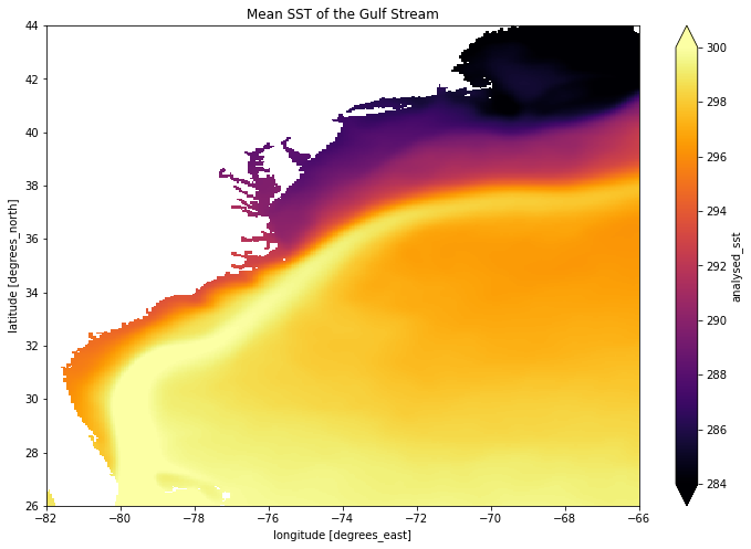
Now let’s take the mean of a year of daily SST data just to clearly see the thermal footprint of the Gulf Stream
fig,ax = plt.subplots(figsize=(12,8))
sst_ds.analysed_sst[0:365].mean(dim='time', skipna=True).plot(ax=ax, vmin=284, vmax=300, cmap='inferno')
ax.set_title('Mean SST of the Gulf Stream')
Text(0.5, 1.0, 'Mean SST of the Gulf Stream')
Sea Wind Speed
As our last dataset we’ll pull in data from EUMETSAT’s Metop-A satellite. ASCAT is a microwave scatterometer designed to measure surface winds over the global ocean and these are 8 day composites of wind speed.
wind_ds = xr.open_zarr('data/winds.zarr')
wind_ds
<xarray.Dataset>
Dimensions: (altitude: 1, latitude: 73, longitude: 65, time: 713)
Coordinates:
* altitude (altitude) float64 10.0
* latitude (latitude) float64 26.0 26.25 26.5 26.75 ... 43.5 43.75 44.0
* longitude (longitude) float64 278.0 278.2 278.5 278.8 ... 293.5 293.8 294.0
* time (time) datetime64[ns] 2010-04-01 2010-04-06 ... 2019-12-30
Data variables:
x_wind (time, altitude, latitude, longitude) float32 dask.array<chunksize=(179, 1, 19, 33), meta=np.ndarray>
y_wind (time, altitude, latitude, longitude) float32 dask.array<chunksize=(179, 1, 19, 33), meta=np.ndarray>- altitude: 1
- latitude: 73
- longitude: 65
- time: 713
- altitude(altitude)float6410.0
- _CoordinateAxisType :
- Height
- _CoordinateZisPositive :
- up
- actual_range :
- [10.0, 10.0]
- axis :
- Z
- fraction_digits :
- 0
- ioos_category :
- Location
- long_name :
- Altitude
- positive :
- up
- standard_name :
- altitude
- units :
- m
array([10.])
- latitude(latitude)float6426.0 26.25 26.5 ... 43.5 43.75 44.0
- _CoordinateAxisType :
- Lat
- actual_range :
- [26.0, 44.0]
- axis :
- Y
- coordsys :
- geographic
- fraction_digits :
- 2
- ioos_category :
- Location
- long_name :
- Latitude
- point_spacing :
- even
- standard_name :
- latitude
- units :
- degrees_north
array([26. , 26.25, 26.5 , 26.75, 27. , 27.25, 27.5 , 27.75, 28. , 28.25, 28.5 , 28.75, 29. , 29.25, 29.5 , 29.75, 30. , 30.25, 30.5 , 30.75, 31. , 31.25, 31.5 , 31.75, 32. , 32.25, 32.5 , 32.75, 33. , 33.25, 33.5 , 33.75, 34. , 34.25, 34.5 , 34.75, 35. , 35.25, 35.5 , 35.75, 36. , 36.25, 36.5 , 36.75, 37. , 37.25, 37.5 , 37.75, 38. , 38.25, 38.5 , 38.75, 39. , 39.25, 39.5 , 39.75, 40. , 40.25, 40.5 , 40.75, 41. , 41.25, 41.5 , 41.75, 42. , 42.25, 42.5 , 42.75, 43. , 43.25, 43.5 , 43.75, 44. ]) - longitude(longitude)float64278.0 278.2 278.5 ... 293.8 294.0
- _CoordinateAxisType :
- Lon
- actual_range :
- [278.0, 294.0]
- axis :
- X
- coordsys :
- geographic
- fraction_digits :
- 2
- ioos_category :
- Location
- long_name :
- Longitude
- point_spacing :
- even
- standard_name :
- longitude
- units :
- degrees_east
array([278. , 278.25, 278.5 , 278.75, 279. , 279.25, 279.5 , 279.75, 280. , 280.25, 280.5 , 280.75, 281. , 281.25, 281.5 , 281.75, 282. , 282.25, 282.5 , 282.75, 283. , 283.25, 283.5 , 283.75, 284. , 284.25, 284.5 , 284.75, 285. , 285.25, 285.5 , 285.75, 286. , 286.25, 286.5 , 286.75, 287. , 287.25, 287.5 , 287.75, 288. , 288.25, 288.5 , 288.75, 289. , 289.25, 289.5 , 289.75, 290. , 290.25, 290.5 , 290.75, 291. , 291.25, 291.5 , 291.75, 292. , 292.25, 292.5 , 292.75, 293. , 293.25, 293.5 , 293.75, 294. ]) - time(time)datetime64[ns]2010-04-01 ... 2019-12-30
array(['2010-04-01T00:00:00.000000000', '2010-04-06T00:00:00.000000000', '2010-04-11T00:00:00.000000000', ..., '2019-12-20T00:00:00.000000000', '2019-12-25T00:00:00.000000000', '2019-12-30T00:00:00.000000000'], dtype='datetime64[ns]')
- x_wind(time, altitude, latitude, longitude)float32dask.array<chunksize=(179, 1, 19, 33), meta=np.ndarray>
Array Chunk Bytes 12.91 MiB 438.41 kiB Shape (713, 1, 73, 65) (179, 1, 19, 33) Count 33 Tasks 32 Chunks Type float32 numpy.ndarray - y_wind(time, altitude, latitude, longitude)float32dask.array<chunksize=(179, 1, 19, 33), meta=np.ndarray>
Array Chunk Bytes 12.91 MiB 438.41 kiB Shape (713, 1, 73, 65) (179, 1, 19, 33) Count 33 Tasks 32 Chunks Type float32 numpy.ndarray
Note above that the longitude goes from 0 to 360 as opposed to -180 through 180 as was the case with the other datasets. We’ll process it here to match the others.
wind_ds['longitude'] = wind_ds['longitude'] -360
This dataset comes with x and y wind speeds, let’s combine them by adding the absolute value of each just to get an idea of total wind speed in a given location.
wind_ds['wind_total'] = abs(wind_ds.y_wind) + abs(wind_ds.y_wind)
Finally let’s add the attribute that this is in meters per second
wind_ds.wind_total.attrs["units"] = 'm/s'
Let’s take a look at the average wind speed across this region.
fig, ax = plt.subplots(figsize=(12,9), subplot_kw=dict(projection=crs.PlateCarree()))
wind_ds.wind_total[0].plot(ax=ax, cmap='coolwarm')
ax.coastlines(resolution='10m')
ax.set_ylim(26,44)
ax.set_xlim(-82,-66)
(-82.0, -66.0)
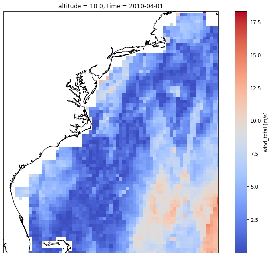
This data is relatively noisy and satellite tracks are somewhat visible, but we’ll resample to monthly below so the noise isn’t as much of an issue. As a test let’s look at the average wind in each month for the entire dataset.
wind_ds.groupby('time.month').median(dim='time').wind_total.hvplot.quadmesh(
'longitude', 'latitude', projection=proj, project=True,
cmap='bwr', dynamic=True, coastline='10m',
frame_width=300, clim=(0,12), rasterize=True)
Gulf Stream front location
Now as a final step in our data prep before we get into the bulk of the analysis we’ll find the location of the front at each time step by finding the 0.25 contour line in sea surface height as done in Andres 2016.
As a quick overview we’re going to:
Get the monthly Gulf Stream front location via the SSH data based on the 25cm contour.
Turn those contours into a geodataframe of monthly front lines
Use these front lines to grab data from all our xarray DataSets to create monthly along-front DataSets
First we’ll resample our SSH data from daily to monthly time steps.
ssh_ds
<xarray.Dataset>
Dimensions: (latitude: 72, longitude: 64, time: 713)
Coordinates:
* latitude (latitude) float32 26.12 26.38 26.62 26.88 ... 43.38 43.62 43.88
* longitude (longitude) float32 -81.88 -81.62 -81.38 ... -66.62 -66.38 -66.12
* time (time) datetime64[ns] 2010-04-01 2010-04-06 ... 2019-12-30
Data variables:
adt (time, latitude, longitude) float64 dask.array<chunksize=(179, 18, 32), meta=np.ndarray>
sla (time, latitude, longitude) float64 dask.array<chunksize=(179, 18, 32), meta=np.ndarray>
ugos (time, latitude, longitude) float64 dask.array<chunksize=(179, 18, 32), meta=np.ndarray>
vgos (time, latitude, longitude) float64 dask.array<chunksize=(179, 18, 32), meta=np.ndarray>- latitude: 72
- longitude: 64
- time: 713
- latitude(latitude)float3226.12 26.38 26.62 ... 43.62 43.88
- _ChunkSizes :
- 50
- _CoordinateAxisType :
- Lat
- axis :
- Y
- bounds :
- lat_bnds
- long_name :
- Latitude
- standard_name :
- latitude
- units :
- degrees_north
- valid_max :
- 89.875
- valid_min :
- -89.875
array([26.125, 26.375, 26.625, 26.875, 27.125, 27.375, 27.625, 27.875, 28.125, 28.375, 28.625, 28.875, 29.125, 29.375, 29.625, 29.875, 30.125, 30.375, 30.625, 30.875, 31.125, 31.375, 31.625, 31.875, 32.125, 32.375, 32.625, 32.875, 33.125, 33.375, 33.625, 33.875, 34.125, 34.375, 34.625, 34.875, 35.125, 35.375, 35.625, 35.875, 36.125, 36.375, 36.625, 36.875, 37.125, 37.375, 37.625, 37.875, 38.125, 38.375, 38.625, 38.875, 39.125, 39.375, 39.625, 39.875, 40.125, 40.375, 40.625, 40.875, 41.125, 41.375, 41.625, 41.875, 42.125, 42.375, 42.625, 42.875, 43.125, 43.375, 43.625, 43.875], dtype=float32) - longitude(longitude)float32-81.88 -81.62 ... -66.38 -66.12
array([-81.875, -81.625, -81.375, -81.125, -80.875, -80.625, -80.375, -80.125, -79.875, -79.625, -79.375, -79.125, -78.875, -78.625, -78.375, -78.125, -77.875, -77.625, -77.375, -77.125, -76.875, -76.625, -76.375, -76.125, -75.875, -75.625, -75.375, -75.125, -74.875, -74.625, -74.375, -74.125, -73.875, -73.625, -73.375, -73.125, -72.875, -72.625, -72.375, -72.125, -71.875, -71.625, -71.375, -71.125, -70.875, -70.625, -70.375, -70.125, -69.875, -69.625, -69.375, -69.125, -68.875, -68.625, -68.375, -68.125, -67.875, -67.625, -67.375, -67.125, -66.875, -66.625, -66.375, -66.125], dtype=float32) - time(time)datetime64[ns]2010-04-01 ... 2019-12-30
array(['2010-04-01T00:00:00.000000000', '2010-04-06T00:00:00.000000000', '2010-04-11T00:00:00.000000000', ..., '2019-12-20T00:00:00.000000000', '2019-12-25T00:00:00.000000000', '2019-12-30T00:00:00.000000000'], dtype='datetime64[ns]')
- adt(time, latitude, longitude)float64dask.array<chunksize=(179, 18, 32), meta=np.ndarray>
- units :
- meters
Array Chunk Bytes 25.07 MiB 805.50 kiB Shape (713, 72, 64) (179, 18, 32) Count 33 Tasks 32 Chunks Type float64 numpy.ndarray - sla(time, latitude, longitude)float64dask.array<chunksize=(179, 18, 32), meta=np.ndarray>
Array Chunk Bytes 25.07 MiB 805.50 kiB Shape (713, 72, 64) (179, 18, 32) Count 33 Tasks 32 Chunks Type float64 numpy.ndarray - ugos(time, latitude, longitude)float64dask.array<chunksize=(179, 18, 32), meta=np.ndarray>
Array Chunk Bytes 25.07 MiB 805.50 kiB Shape (713, 72, 64) (179, 18, 32) Count 33 Tasks 32 Chunks Type float64 numpy.ndarray - vgos(time, latitude, longitude)float64dask.array<chunksize=(179, 18, 32), meta=np.ndarray>
Array Chunk Bytes 25.07 MiB 805.50 kiB Shape (713, 72, 64) (179, 18, 32) Count 33 Tasks 32 Chunks Type float64 numpy.ndarray
ssh_ds_monthly = ssh_ds.resample(time="1M").mean()
ssh_ds_monthly.adt.attrs["units"] = 'meters'
Then we’ll run the subpixel_contours() function which takes in an xarray DataArray and related geospatial metadata and returns a geodataframe of the contours at each time step.
To do this we need to define an affine transformation for the SSH data since it doesn’t exist in the dataset currently. Learn more here. The basic format of an affine transformation is (a, b, c, d, e, f):
a = width of a pixel
b = row rotation (typically zero)
c = x-coordinate of the upper-left corner of the upper-left pixel
d = column rotation (typically zero)
e = height of a pixel (typically negative)
f = y-coordinate of the of the upper-left corner of the upper-left pixel
We define the CRS as 4326 which is WGS84 so it just uses lat and lon. Thus the width of a pixel is .25 degrees.
ssh_affine = Affine(0.25, 0.0, -81.875-.25/2, 0.0, 0.25, 26.125-.25/2)
ssh_affine
Affine(0.25, 0.0, -82.0,
0.0, 0.25, 26.0)
# this function needs all the data in memory so load it in
ssh_ds_monthly.adt.load()
gdf = subpixel_contours(ssh_ds_monthly.adt, [0.25], crs='EPSG:4326', min_vertices=50, affine=ssh_affine, verbose=True)
Operating in single z-value, multiple arrays mode
gdf.plot()
plt.title('All front lines from subpixel_contours()')
plt.xlabel('longitude')
plt.ylabel('latitude')
Text(101.4562601240053, 0.5, 'latitude')
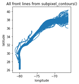
As can be seen above, this approach to finding the front does pick up a few anomalous frontal eddies in the South Atlantic Bight so we’re going to require all lines pass south of 28 degrees latitude and east of -70 degrees longitude.
print(len(gdf))
gdf = gdf.cx[:,26:28].cx[-70:-66,:]
print(len(gdf))
gdf.plot()
plt.title('Filtered front lines')
plt.xlabel('longitude')
plt.ylabel('latitude')
117
104
Text(106.10908404930032, 0.5, 'latitude')
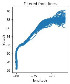
Note that we lose 13 months out of the 10 years of data because of this constraint.
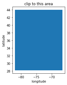
And finally because the Gulf Stream is so close to the Florida coast around 26 degrees north, we’ll clip it to 28 N and above and to west of -66.5 longitude so it isn’t on the edge of our data.
# Create a custom polygon to clip with
polygon = Polygon([(-82, 28.2), (-82, 44), (-66.5, 44), (-66.5, 28.2), (-82, 28.2)])
poly_gdf = gpd.GeoDataFrame([1], geometry=[polygon], crs=gdf.crs)
poly_gdf.plot()
plt.title('clip to this area')
plt.xlabel('longitude')
plt.ylabel('latitude')
Text(111.47327640825279, 0.5, 'latitude')
gdf = gpd.clip(gdf, polygon)
gdf.plot()
plt.title('Filtered and clipped front lines')
plt.xlabel('longitude')
plt.ylabel('latitude')
Text(95.04134645269737, 0.5, 'latitude')
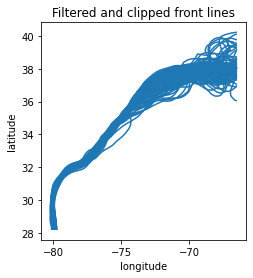
That seems to nicely solve the issue
gdf.hvplot.paths('Longitude', 'Latitude', geo=True, color='red', alpha=0.8,
tiles='ESRI', frame_width=500, title='filtered and clipped front lines')
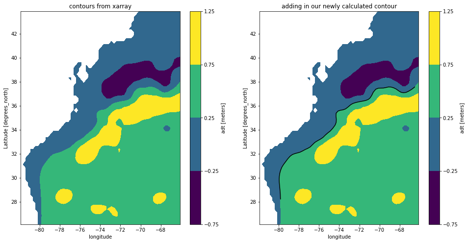
Let’s quickly check to see if our contour matches exactly with the contours from the xarray contour function.
fig,ax= plt.subplots(1,2, figsize=(16,8))
ssh_ds_monthly.adt[0].plot.contourf(ax=ax[0], vmin=-1,vmax=1,center=0.25,levels=5)
ssh_ds_monthly.adt[0].plot.contourf(ax=ax[1], vmin=-1,vmax=1,center=0.25,levels=5)
gdf.head(1).plot(ax=ax[1], color='black')
ax[0].set_title('contours from xarray')
ax[1].set_title('adding in our newly calculated contour')
Text(0.5, 1.0, 'adding in our newly calculated contour')
Selecting data along the front
Now let’s turn our contour lines into points so that we can grab the xarray values at each point.
lon,lat = gdf.iloc[0].geometry.coords.xy
df = pd.DataFrame(list(zip(lat,lon)), columns=['lat', 'lon'])
points_gdf = gpd.GeoDataFrame(
df, geometry=gpd.points_from_xy(df.lon, df.lat))
points_gdf.hvplot.points(geo=True, color='red', alpha=0.8,
tiles='ESRI', frame_width=500, title='points from a contour line')
These points are irregularly spaced as a product of the contour algorithm and we want to have them all regularly spaced along the line. So we’ll make 90 evenly spaced points on each front line.
We also want a coastal line and an open ocean line that run parallel to the front line but allow us to compare differences along the front and nearby waters. We’ll offset lines ~20 km from our front line on either side.
points_list = []
points_list_coastal = []
points_list_sargasso = []
# number of points along the line
n = 90
for i, line in gdf.iterrows():
# create equally spaced points along the line
distances = np.linspace(0, line.geometry.length, n)
# turn them into shapely points
points = [line.geometry.interpolate(distance) for distance in distances]
# join them into multipoint objects
multipoint = unary_union(points)
# move north and west
coastal_points = []
for point in points:
coastal_points.append(transform(lambda x, y: (x-0.2, y+0.2), point))
multipoint_coastal = unary_union(coastal_points)
# move south and east
sargasso_points = []
for point in points:
sargasso_points.append(transform(lambda x, y: (x+0.2, y-0.2), point))
multipoint_sargasso = unary_union(sargasso_points)
points_list.append(multipoint)
points_list_coastal.append(multipoint_coastal)
points_list_sargasso.append(multipoint_sargasso)
Turn those points into a geodataframe
points_gdf = gpd.GeoDataFrame(gdf['time'], geometry=points_list)
points_gdf.head()
| time | geometry | |
|---|---|---|
| 0 | 2010-04-30 | MULTIPOINT (-79.94784 29.89639, -79.94212 29.6... |
| 1 | 2010-05-31 | MULTIPOINT (-79.95294 29.63065, -79.94815 29.4... |
| 2 | 2010-06-30 | MULTIPOINT (-80.03268 29.73742, -80.02246 29.5... |
| 3 | 2010-07-31 | MULTIPOINT (-79.99216 29.88542, -79.99056 29.6... |
| 4 | 2010-08-31 | MULTIPOINT (-80.02057 29.71148, -80.01368 29.9... |
coastal_points_gdf = gpd.GeoDataFrame(gdf['time'], geometry=points_list_coastal)
coastal_points_gdf.head()
| time | geometry | |
|---|---|---|
| 0 | 2010-04-30 | MULTIPOINT (-80.14784 30.09639, -80.14212 29.8... |
| 1 | 2010-05-31 | MULTIPOINT (-80.15294 29.83065, -80.14815 29.6... |
| 2 | 2010-06-30 | MULTIPOINT (-80.23268 29.93742, -80.22246 29.7... |
| 3 | 2010-07-31 | MULTIPOINT (-80.19216 30.08542, -80.19056 29.8... |
| 4 | 2010-08-31 | MULTIPOINT (-80.22057 29.91148, -80.21368 30.1... |
sargasso_points_gdf = gpd.GeoDataFrame(gdf['time'], geometry=points_list_sargasso)
sargasso_points_gdf.head()
| time | geometry | |
|---|---|---|
| 0 | 2010-04-30 | MULTIPOINT (-79.74784 29.69639, -79.74212 29.4... |
| 1 | 2010-05-31 | MULTIPOINT (-79.75294 29.43065, -79.74815 29.2... |
| 2 | 2010-06-30 | MULTIPOINT (-79.83268 29.53742, -79.82246 29.3... |
| 3 | 2010-07-31 | MULTIPOINT (-79.79216 29.68542, -79.79056 29.4... |
| 4 | 2010-08-31 | MULTIPOINT (-79.82057 29.51148, -79.81368 29.7... |
Display 10 frontal lines against the backdrop of SSH
ssh_ds_monthly.adt[0].hvplot.quadmesh(
'longitude', 'latitude',
cmap='bwr', dynamic=True, coastline='10m',
frame_width=300, clim=(-1,1), datashade=False, title='evenly spaced points from front contours') * \
points_gdf.head(10).hvplot.points(geo=True, color='black', alpha=0.7)
Now let’s check out the coastal, frontal, and sargasso lines together
ssh_ds_monthly.adt[0].hvplot.quadmesh(
'longitude', 'latitude',
cmap='bwr', dynamic=True, coastline='10m',
frame_width=300, clim=(-1,1), datashade=False, title='points from coastal, front, and sargasso lines') * \
coastal_points_gdf.head(1).hvplot.points(geo=True, color='green', alpha=0.7, label='coastal') * \
sargasso_points_gdf.head(1).hvplot.points(geo=True, color='blue', alpha=0.7, label='sargasso') * \
points_gdf.head(1).hvplot.points(geo=True, color='black', alpha=0.7, label='front')
Now let’s run this same process but for each time step.
Create an xarray DataArray each day and each frontal line
# there could be a better way to do this than iterating through the gdf
x_list = []
y_list = []
for i in range(len(points_gdf)):
points = np.array([[p.x, p.y] for p in points_gdf.iloc[i].geometry])
x_list.append(points[:,0])
y_list.append(points[:,1])
x_list = np.array(x_list)
y_list = np.array(y_list)
x_list.shape, y_list.shape
((104, 90), (104, 90))
Using those points and time steps let’s create a few DataArrays that we’ll used to select from the primary DataSets
target_lon = xr.DataArray(x_list, dims=["time", "points"])
target_lat = xr.DataArray(y_list, dims=["time", "points"])
target_time = xr.DataArray(pd.to_datetime(points_gdf['time']).values, dims="time")
target_lat
<xarray.DataArray (time: 104, points: 90)>
array([[29.89639445, 29.68377097, 30.10882517, ..., 37.34995009,
37.46070548, 37.58056103],
[29.63065387, 29.42518819, 29.83596842, ..., 37.67276385,
37.63860507, 37.60508772],
[29.73741752, 29.51572437, 29.95907477, ..., 38.36849948,
38.5451644 , 38.71095009],
...,
[29.68460092, 29.93209271, 29.43725985, ..., 40.14658275,
40.18599803, 40.21366327],
[29.45212053, 29.66378186, 29.24154626, ..., 38.08109788,
38.08500311, 38.1004156 ],
[29.66961262, 29.8804883 , 29.458972 , ..., 37.86050383,
37.84379338, 37.83656502]])
Dimensions without coordinates: time, points- time: 104
- points: 90
- 29.9 29.68 30.11 29.47 29.26 30.32 ... 37.93 37.89 37.86 37.84 37.84
array([[29.89639445, 29.68377097, 30.10882517, ..., 37.34995009, 37.46070548, 37.58056103], [29.63065387, 29.42518819, 29.83596842, ..., 37.67276385, 37.63860507, 37.60508772], [29.73741752, 29.51572437, 29.95907477, ..., 38.36849948, 38.5451644 , 38.71095009], ..., [29.68460092, 29.93209271, 29.43725985, ..., 40.14658275, 40.18599803, 40.21366327], [29.45212053, 29.66378186, 29.24154626, ..., 38.08109788, 38.08500311, 38.1004156 ], [29.66961262, 29.8804883 , 29.458972 , ..., 37.86050383, 37.84379338, 37.83656502]])
Now let’s resample all the datasets to monthly averages
We also need to specify the units since these operations may potentially change them and so theyr’re removed by default.
chla_ds_monthly = chla_ds.resample(time="1M").mean()
chla_ds_monthly.chlor_a.attrs["units"] = 'mg m^-3'
sst_ds_monthly = sst_ds.resample(time="1M").mean()
sst_ds_monthly.analysed_sst.attrs["units"] = 'Kelvin'
wind_ds_monthly = wind_ds.resample(time="1M").mean()
wind_ds_monthly.wind_total.attrs["units"] = 'm/s'
And now run select the nearest neighbor in time and space to each point
ssh_ds_frontal = ssh_ds_monthly.adt.sel(time=target_time, latitude=target_lat, longitude=target_lon, method="nearest")
chla_ds_frontal = chla_ds_monthly.chlor_a.sel(time=target_time, lat=target_lat, lon=target_lon, method="nearest")
sst_ds_frontal = sst_ds_monthly.analysed_sst.sel(time=target_time, lat=target_lat, lon=target_lon, method="nearest")
wind_ds_frontal = wind_ds_monthly.wind_total.sel(time=target_time, latitude=target_lat, longitude=target_lon, method="nearest")
As a sanity check, let’s take a look at the SSH along the points in this front line which was derived from the 0.25 contour line just to ensure that is is approximately 0.25 still.
ssh_ds_frontal[0].plot()
plt.title('SSH at points processed from 0.25m contour line')
Text(0.5, 1.0, 'SSH at points processed from 0.25m contour line')
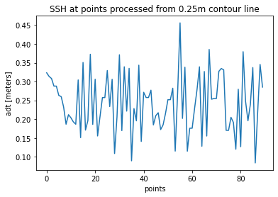
Note that this does introduce a little error since we’ve interpolated the contour and it isn’t exactly on the .25m line
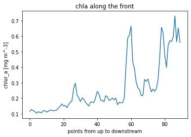
chla_ds_frontal[0].plot()
plt.title('chla along the front')
plt.xlabel('points from up to downstream')
Text(0.5, 0, 'points from up to downstream')
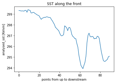
sst_ds_frontal[0].plot()
plt.title('SST along the front')
plt.xlabel('points from up to downstream')
Text(0.5, 0, 'points from up to downstream')
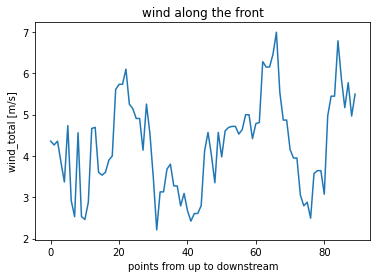
wind_ds_frontal[0].plot()
plt.title('wind along the front')
plt.xlabel('points from up to downstream')
Text(0.5, 0, 'points from up to downstream')
And finally we want to do the exact same thing for the coastal and sargasso lines. We’ll write a quick function for this and apply it to the coastal and sargasso lines.
def frontal_dataset_generation(line_gdf, ssh_monthly, chla_monthly, sst_monthly, wind_monthly):
x_list = []
y_list = []
for i in range(len(line_gdf)):
points = np.array([[p.x, p.y] for p in line_gdf.iloc[i].geometry])
x_list.append(points[:,0])
y_list.append(points[:,1])
x_list = np.array(x_list)
y_list = np.array(y_list)
target_lon = xr.DataArray(x_list, dims=["time", "points"])
target_lat = xr.DataArray(y_list, dims=["time", "points"])
target_time = xr.DataArray(pd.to_datetime(points_gdf['time']).values, dims="time")
ssh_line = ssh_monthly.adt.sel(time=target_time, latitude=target_lat, longitude=target_lon, method="nearest")
chla_line = chla_monthly.chlor_a.sel(time=target_time, lat=target_lat, lon=target_lon, method="nearest")
sst_line = sst_monthly.analysed_sst.sel(time=target_time, lat=target_lat, lon=target_lon, method="nearest")
wind_line = wind_monthly.wind_total.sel(time=target_time, latitude=target_lat, longitude=target_lon, method="nearest")
return(ssh_line,chla_line,sst_line,wind_line)
ssh_ds_sargasso,chla_ds_sargasso,sst_ds_sargasso,wind_ds_sargasso = frontal_dataset_generation(sargasso_points_gdf, ssh_ds_monthly, chla_ds_monthly, sst_ds_monthly, wind_ds_monthly)
ssh_ds_coastal,chla_ds_coastal,sst_ds_coastal,wind_ds_coastal = frontal_dataset_generation(coastal_points_gdf, ssh_ds_monthly, chla_ds_monthly, sst_ds_monthly, wind_ds_monthly)
Now our data is ready let’s analyze!
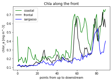
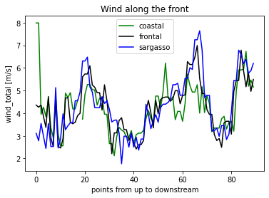
Let’s just quickly look at a single time step from each dataset. We’ll represent the coastal line with green, frontal line with black, and open ocean (sargasso sea) line with blue.
fig, ax = plt.subplots()
sst_ds_coastal[0].plot(ax=ax, color='green', label='coastal')
sst_ds_frontal[0].plot(ax=ax, color='black', label='frontal')
sst_ds_sargasso[0].plot(ax=ax, color='blue', label='sargasso')
ax.legend(loc='best')
plt.title('SST along the front')
plt.xlabel('points from up to downstream')
Text(0.5, 0, 'points from up to downstream')

fig, ax = plt.subplots()
chla_ds_coastal[0].plot(ax=ax, color='green', label='coastal')
chla_ds_frontal[0].plot(ax=ax, color='black', label='frontal')
chla_ds_sargasso[0].plot(ax=ax, color='blue', label='sargasso')
ax.legend(loc='best')
plt.title('Chla along the front')
plt.xlabel('points from up to downstream')
Text(0.5, 0, 'points from up to downstream')
fig, ax = plt.subplots()
wind_ds_coastal[0].plot(ax=ax, color='green', label='coastal')
wind_ds_frontal[0].plot(ax=ax, color='black', label='frontal')
wind_ds_sargasso[0].plot(ax=ax, color='blue', label='sargasso')
ax.legend(loc='best')
plt.title('Wind along the front')
plt.xlabel('points from up to downstream')
Text(0.5, 0, 'points from up to downstream')
Data processing and analysis
Now we’ve made it through all the data processing steps and can begin analysis of this frontal dataset we’ve created.
Visualizing all datasets
First let’s just examine the data quickly to ensure there isn’t anything obviously erroneous and to see if we find any clear trends. These charts show chla, SST, and SSH with the front plotted over top of them for all of 2018.
# add a datetime object to the front gdf so that we can select by time
points_gdf['dt_time'] = pd.to_datetime(points_gdf['time'])
for i in range(12,24):
fig,ax = plt.subplots(1,4,figsize=(30,8))
# there must be a better way to convert from cftime to datetime in xarray
current_dt = datetime.datetime.strptime(str(sst_ds_monthly.time[i].dt.strftime("%Y, %m, %d").values),"%Y, %m, %d")
sst_ds_monthly.analysed_sst[i].plot(ax=ax[1], cmap='inferno', vmin=290, vmax=304)
# have to select from these based on SST because they are much longer time series
chla_ds_monthly.chlor_a.sel(time=current_dt, method="nearest").plot(ax=ax[0], cmap='jet', norm=LogNorm(vmin=0.01, vmax=10))
ssh_ds_monthly.adt.sel(time=current_dt, method="nearest").plot(ax=ax[2], cmap='bwr', vmin=-1, vmax=1)
wind_ds_monthly.wind_total.sel(time=current_dt, method="nearest").plot(ax=ax[3], cmap='coolwarm', vmin=0, vmax=9)
month_gdf = points_gdf[points_gdf['dt_time'] == current_dt]
month_gdf.plot(ax=ax[0], color='black', alpha=0.9, markersize=10)
month_gdf.plot(ax=ax[1], color='black', alpha=0.9, markersize=10)
month_gdf.plot(ax=ax[2], color='black', alpha=0.9, markersize=10)
month_gdf.plot(ax=ax[3], color='black', alpha=0.9, markersize=10)
plt.show()
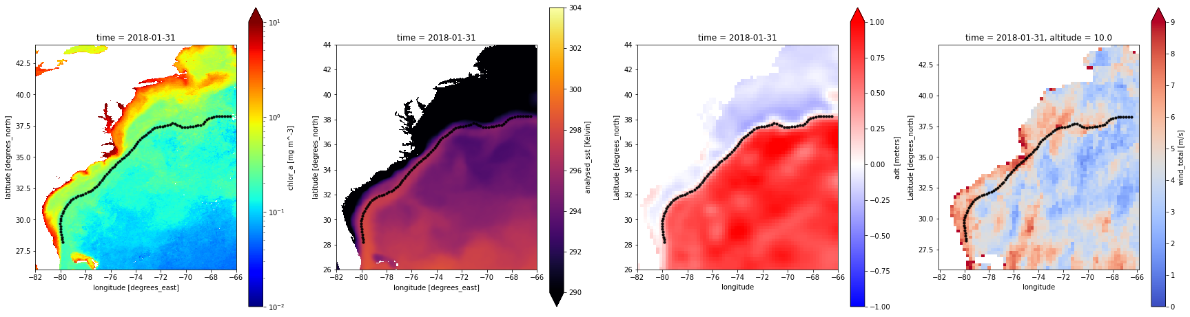
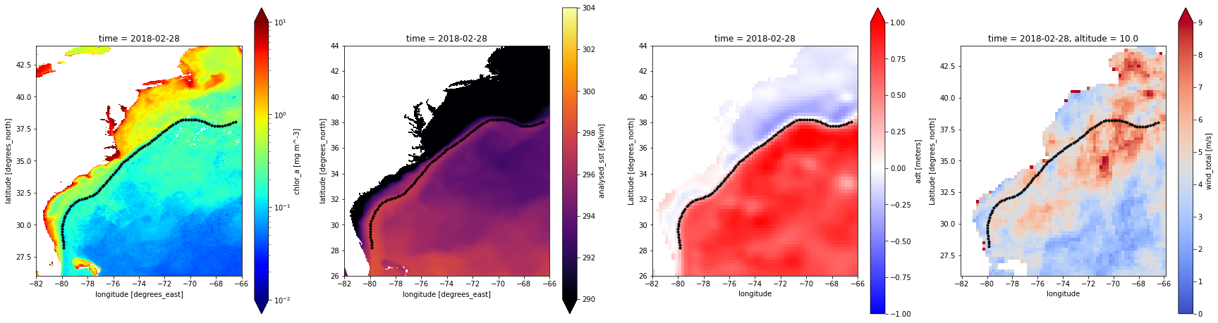
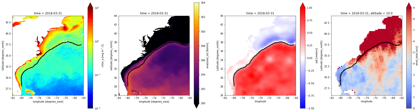
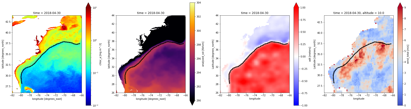
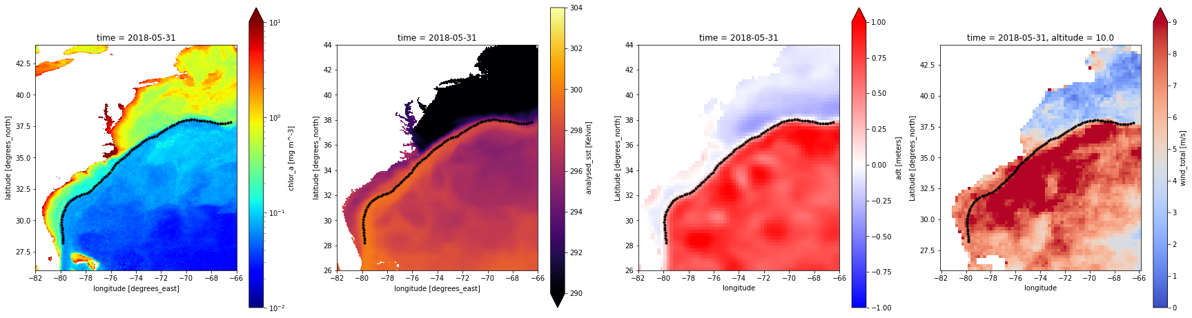
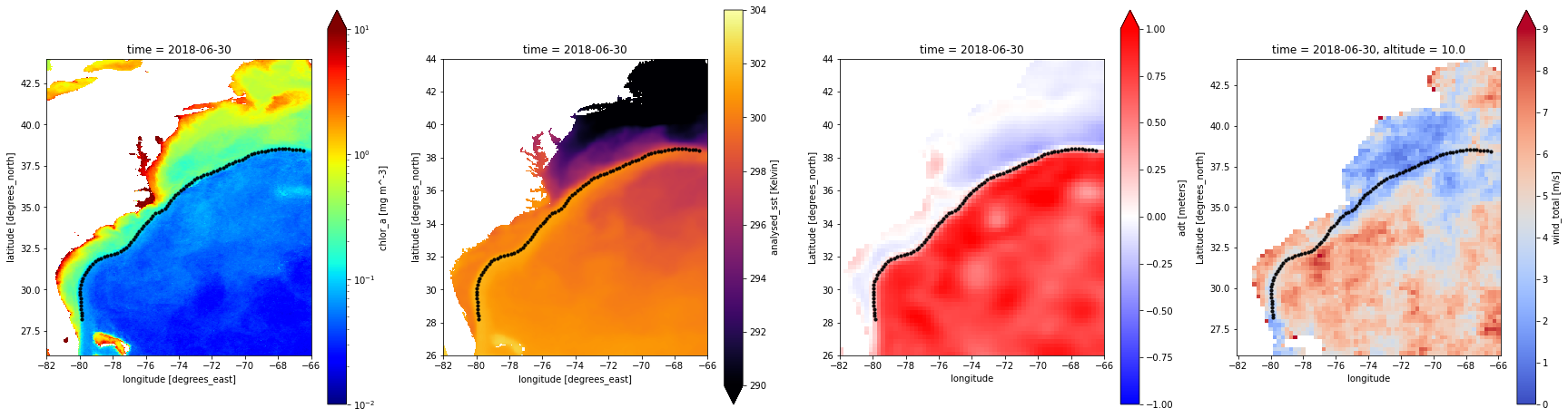
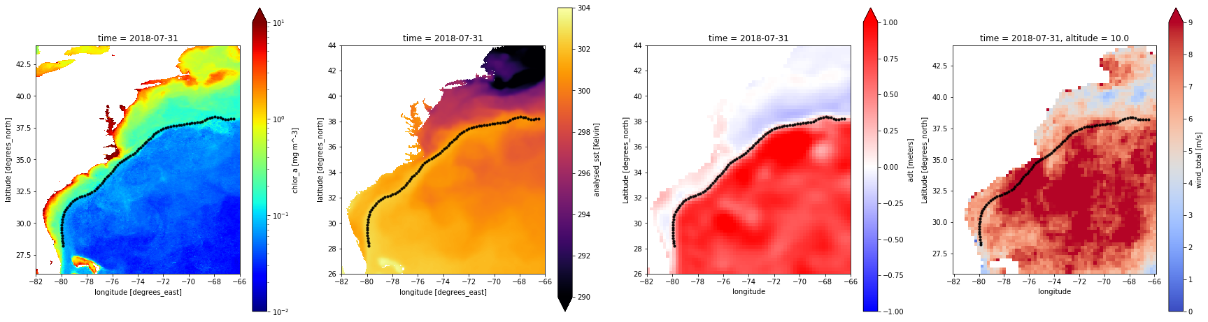
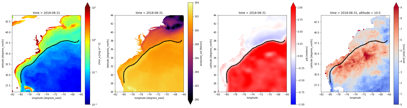
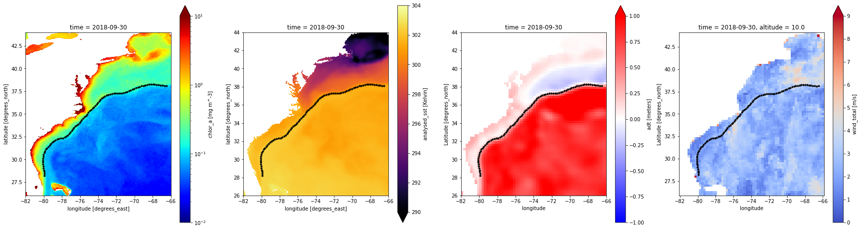
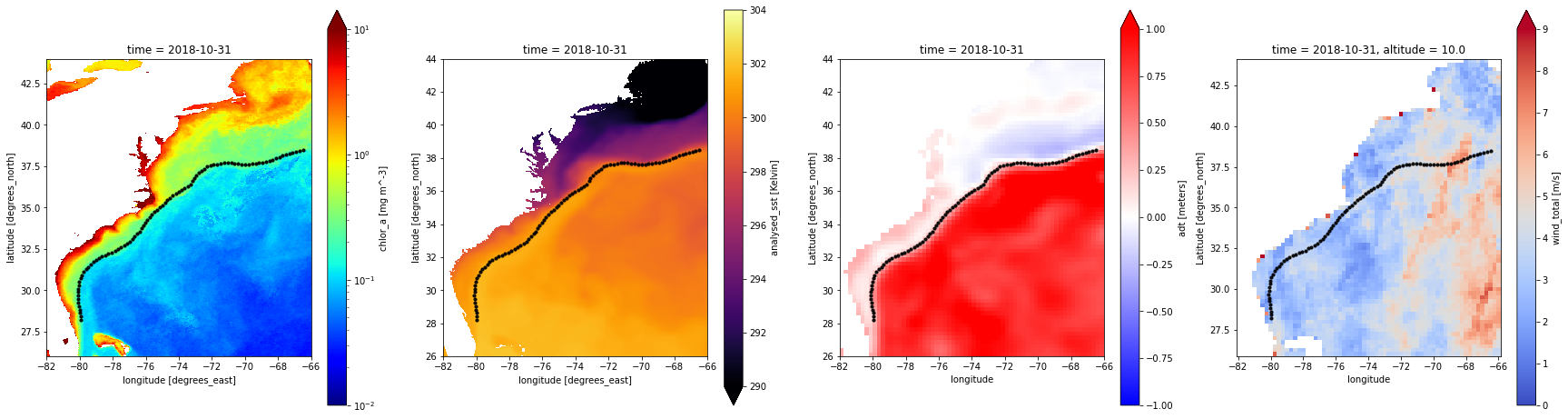
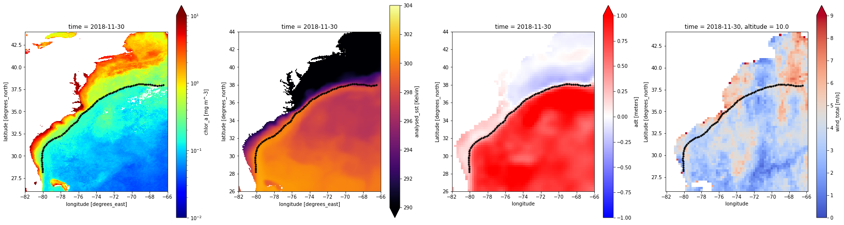
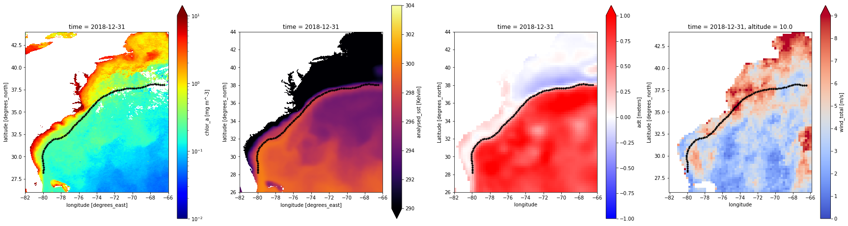
These figures really make it clear how much the GS is major boundary between the coastal and the open ocean ecosystems.
A large increase in chlorophyll-a beyond the Gulf Stream front, aka in the Sargasso Sea, is evident from late fall to early spring. The spring bloom in the North Atlantic is also clear where it peaks in April and May. Note that the scale is logarithmic so the red colors are two orders of magnitude highers than teal.
The SST data matches what one might expect, decreasing throughout the winter and increasing in summer with the Gulf Stream itself staying as the warmest water throughout all seasons. We can also see a few eddies in SST and SSH even though this data is resampled to monthly time steps.
Seasonality along the Gulf Stream
Now let’s look at the chla on the front itself over time. Make sure you use the scroll bar to explore the data over time.
chla_ds_frontal.hvplot.line(x='points', value_label='time', ylim=(0,1), color='black', label='frontal') * \
chla_ds_coastal.hvplot.line(x='points', value_label='time', ylim=(0,1), color='green', label='coastal') * \
chla_ds_sargasso.hvplot.line(x='points', value_label='time', ylim=(0,1), color='blue', label='sargasso', xlabel='points up to downstream')
Note sustained spike in chla off Cape Hatteras near the front on the coastal side.
The spring bloom is also noticable in all three lines from points 60 to 90.
Moving on here to SST:
sst_ds_frontal.hvplot.line(x='points', value_label='time', ylim=(290,304), color='black', label='frontal') * \
sst_ds_coastal.hvplot.line(x='points', value_label='time', ylim=(290,304), color='green', label='coastal') *\
sst_ds_sargasso.hvplot.line(x='points', value_label='time', ylim=(290,304), color='blue', label='sargasso', xlabel='points up to downstream')
SST follows a relatively predictable pattern with most variation seemingly tied to seasonality.
Moving to wind now:
wind_ds_coastal.hvplot.line(x='points', value_label='time', ylim=(0,15), xlim=(1,90), color='green', label='coastal') * \
wind_ds_frontal.hvplot.line(x='points', value_label='time', ylim=(0,15), xlim=(1,90), color='black', label='frontal') * \
wind_ds_sargasso.hvplot.line(x='points', value_label='time', ylim=(0,15), xlim=(1,90), color='blue', label='sargasso', xlabel='points up to downstream')
Winds are highly variable, but show some seasonality with an increase in the winter. This is a part of most descriptions of the spring bloom, winter storms drive mixing which adds sufficient nutrients into the euphotic zone for the major spring increase once sunlight/stratification returns.
You can see some hints at the dynamics at play in these plots, but let’s look at it all at once via a Hovmöller diagram with the spatial points on the x axis, time on the y, and the color showing the value of the variable.
In these plots Point 0 is the furthest point upstream around Florida and Point 90 is downstream in the North Atlantic.
fig, ax = plt.subplots(1,3,figsize=(20,8))
# cut the last two dates off so it doesn't strech it to 2020
chla_ds_coastal[:-2].plot(ax=ax[0],norm=LogNorm(vmin=0.05, vmax=5), cmap='jet', xlim=(2,90))
chla_ds_frontal[:-2].plot(ax=ax[1],norm=LogNorm(vmin=0.05, vmax=5), cmap='jet', xlim=(2,90))
chla_ds_sargasso[:-2].plot(ax=ax[2],norm=LogNorm(vmin=0.05, vmax=5), cmap='jet', xlim=(2,90))
ax[0].set_title('coastal chla')
ax[0].set_xlabel('points up to downstream')
ax[1].set_title('frontal chla')
ax[1].set_xlabel('points up to downstream')
ax[2].set_title('sargasso chla')
ax[2].set_xlabel('points up to downstream')
fig.tight_layout()
plt.show()
Let’s look one more time at chla over just a few years
fig, ax = plt.subplots(1,3,figsize=(20,8))
# cut the last two dates off so it doesn't strech it to 2020
chla_ds_coastal[:36].plot(ax=ax[0],norm=LogNorm(vmin=0.05, vmax=5), cmap='jet', xlim=(2,90))
chla_ds_frontal[:36].plot(ax=ax[1],norm=LogNorm(vmin=0.05, vmax=5), cmap='jet', xlim=(2,90))
chla_ds_sargasso[:36].plot(ax=ax[2],norm=LogNorm(vmin=0.05, vmax=5), cmap='jet', xlim=(2,90))
ax[0].set_title('coastal chla')
ax[0].set_xlabel('points up to downstream')
ax[1].set_title('frontal chla')
ax[1].set_xlabel('points up to downstream')
ax[2].set_title('sargasso chla')
ax[2].set_xlabel('points up to downstream')
fig.tight_layout()
plt.show()
fig, ax = plt.subplots(1,3,figsize=(20,5))
sst_ds_coastal.plot(ax=ax[0], vmin=293, vmax=303, cmap='inferno', xlim=(2,90))
sst_ds_frontal.plot(ax=ax[1],vmin=293, vmax=303, cmap='inferno', xlim=(2,90))
sst_ds_sargasso.plot(ax=ax[2],vmin=293, vmax=303, cmap='inferno', xlim=(2,90))
ax[0].set_title('coastal SST')
ax[0].set_xlabel('points up to downstream')
ax[1].set_title('frontal SST')
ax[1].set_xlabel('points up to downstream')
ax[2].set_title('sargasso SST')
ax[2].set_xlabel('points up to downstream')
fig.tight_layout()
plt.show()
fig, ax = plt.subplots(1,3,figsize=(20,8))
wind_ds_coastal.plot(ax=ax[0], vmin=3, vmax=12, cmap='coolwarm', xlim=(2,90))
wind_ds_frontal.plot(ax=ax[1],vmin=3, vmax=12, cmap='coolwarm', xlim=(2,90))
wind_ds_sargasso.plot(ax=ax[2],vmin=3, vmax=12, cmap='coolwarm', xlim=(2,90))
ax[0].set_title('coastal wind')
ax[0].set_xlabel('points up to downstream')
ax[1].set_title('frontal wind')
ax[1].set_xlabel('points up to downstream')
ax[2].set_title('sargasso wind')
ax[2].set_xlabel('points up to downstream')
fig.tight_layout()
plt.show()
The intense seasonality of SST is clearly apparent and a dominant factor but chla is much more variable, influenced by more than just the temperature and light exposure.
We can show more quantatively that chla is more variable via the coefficient of variation here.
For reference point 20 is approx Charleston SC, point 40 is approx Cape Lookout NC, point 50 is Cape Hatteras NC, and point 60 and beyond are offshore.
(chla_ds_coastal.std(dim='time')/chla_ds_frontal.mean(dim='time')).plot(xlim=(2,90), color='green',label='coastal',)
(chla_ds_frontal.std(dim='time')/chla_ds_frontal.mean(dim='time')).plot(xlim=(2,90), color='black',label='frontal',)
(chla_ds_sargasso.std(dim='time')/chla_ds_frontal.mean(dim='time')).plot(xlim=(2,90), color='blue', label='sargasso')
plt.title('coefficient of variation of chla at each point')
plt.legend()
plt.xlabel('points up to downstream')
plt.ylabel('coefficient of variation of chlor_a')
plt.ylim(0,3)
You can see that right around point 45 which is nearshore and near Cape Hatteras is where the physical structure of GS connects with an area that has major bursts of productivity.
(sst_ds_coastal.std(dim='time')/sst_ds_frontal.mean(dim='time')).plot(xlim=(2,90), color='green',label='coastal')
(sst_ds_frontal.std(dim='time')/sst_ds_frontal.mean(dim='time')).plot(xlim=(2,90), color='black',label='frontal')
(sst_ds_sargasso.std(dim='time')/sst_ds_frontal.mean(dim='time')).plot(xlim=(2,90), color='blue',label='sargasso')
plt.title('coefficient of variation of SST at each point')
plt.legend()
plt.xlabel('points up to downstream')
plt.ylabel('coefficient of variation of SST')
#plt.ylim(0,3)
As you can see chla is 50-100 times more variable than SST and the temperature of the front is much more variable downstream which makes sense given the more intense seasonality there.
The full time series
Now let’s look at the full time series of chla in the various segments. First we’ll look at the offshore segment in the North Atlantic.
fig,ax = plt.subplots(figsize=(12,7))
chla_ds_frontal[:,60:].median('points').plot(ax=ax,color='black', label='frontal')
chla_ds_coastal[:,60:].median('points').plot(ax=ax,color='green', label='coastal')
chla_ds_sargasso[:,60:].median('points').plot(ax=ax,color='blue', label='sargasso')
ax.set_ylim(0,1.2)
ax.set_title('avg chla of offshore section over time')
ax.set_ylabel('chlor_a [mg m^-3]')
ax.legend()
And then the section around Cape Lookout and Cape Hatteras
fig,ax = plt.subplots(figsize=(12,7))
chla_ds_frontal[:,40:50].median('points').plot(ax=ax,color='black', label='frontal')
chla_ds_coastal[:,40:50].median('points').plot(ax=ax,color='green', label='coastal')
chla_ds_sargasso[:,40:50].median('points').plot(ax=ax,color='blue', label='sargasso')
ax.set_ylim(0,1.2)
ax.set_title('avg chla of Cape Hatteras section over time')
ax.set_ylabel('chlor_a [mg m^-3]')
ax.legend()
fig,ax = plt.subplots(figsize=(12,7))
chla_ds_frontal[:,20:40].median('points').plot(ax=ax,color='black', label='frontal')
chla_ds_coastal[:,20:40].median('points').plot(ax=ax,color='green', label='coastal')
chla_ds_sargasso[:,20:40].median('points').plot(ax=ax,color='blue', label='sargasso')
ax.set_ylim(0,1.2)
ax.set_title('avg chla of South Atlantic Bight section over time')
ax.set_ylabel('chlor_a [mg m^-3]')
ax.legend()
A couple major takeaways from this analysis thus far.
The offshore region further downstream seems to have a major increase in the spring - the well studied spring bloom - and the region further south (upstream) around the South Atlantic Bight (SAB) has a relatively large increase throughout the whole winter starting mid fall and staying high until the spring. The region around Cape Hatteras falls in the middle of these two patterns but with generally higher chla, particularly on the coastal side, which makes sense given its proximity to the coast in this region and generally large outflows from Pamlico Sound and Chesapeake Bay injecting nutrients into the water. It is also worth noting that the more northerly section of the front does seem to have a more notable dip mid-winter, possibly when light begins to be limiting, and this is not as pronounced in the southerly section of the front. Though the light difference is not extreme, it is 9.5 hours on the winter solstice at 37 degrees N and 10.6 at 27 degrees N.
fig,ax = plt.subplots(figsize=(12,7))
chla_ds_frontal.median('points').plot(ax=ax,color='black', label='frontal')
chla_ds_coastal.median('points').plot(ax=ax,color='green', label='coastal')
chla_ds_sargasso.median('points').plot(ax=ax,color='blue', label='sargasso')
ax.set_ylim(0,0.6)
ax.set_title('avg chla of entire line over time')
ax.set_ylabel('chlor_a [mg m^-3]')
ax.legend()
It is interesting to see that for nearly all of the Gulf Stream from from Florida out into the North Atlantic there is a fall bloom that is comparable or greater than the spring bloom and this is true of both sides of the front. It decreases around mid-winter, likely due to light limitation (depending on the region), and then increases again as light begins to increase. At least that is our general idea!
Inspecting the SST data here in the same fashion to see if there are any surprising trends.
fig,ax = plt.subplots(figsize=(12,7))
sst_ds_frontal[:,60:].mean('points').plot(ax=ax,color='black', label='frontal')
sst_ds_coastal[:,60:].mean('points').plot(ax=ax,color='green', label='coastal')
sst_ds_sargasso[:,60:].mean('points').plot(ax=ax,color='blue', label='sargasso')
ax.set_ylim(290,303)
ax.set_title('avg SST of offshore section over time')
ax.set_ylabel('SST [Kelvin]')
ax.legend()
fig,ax = plt.subplots(figsize=(12,7))
sst_ds_frontal[:,40:50].mean('points').plot(ax=ax,color='black', label='frontal')
sst_ds_coastal[:,40:50].mean('points').plot(ax=ax,color='green', label='coastal')
sst_ds_sargasso[:,40:50].mean('points').plot(ax=ax,color='blue', label='sargasso')
ax.set_ylim(290,303)
ax.set_ylabel('SST [Kelvin]')
ax.set_title('avg SST of Cape Hatteras section over time')
ax.legend()
fig,ax = plt.subplots(figsize=(12,7))
sst_ds_frontal[:,20:40].mean('points').plot(ax=ax,color='black', label='frontal')
sst_ds_coastal[:,20:40].mean('points').plot(ax=ax,color='green', label='coastal')
sst_ds_sargasso[:,20:40].mean('points').plot(ax=ax,color='blue', label='sargasso')
ax.set_ylim(290,303)
ax.set_title('avg SST of South Atlantic Bight section over time')
ax.set_ylabel('SST [Kelvin]')
ax.legend()
Finally let’s see how the wind behaves in relation to chla along the front
fig,ax = plt.subplots(figsize=(12,7))
wind_ds_frontal[:,:,60:].median('points').plot(ax=ax,color='black', label='frontal')
wind_ds_coastal[:,:,60:].median('points').plot(ax=ax,color='green', label='coastal')
wind_ds_sargasso[:,:,60:].median('points').plot(ax=ax,color='blue', label='sargasso')
ax.set_ylim(0,10)
ax.set_title('avg wind of offshore section over time')
ax.set_ylabel('Wind Total [m/s]')
ax.legend()
fig,ax = plt.subplots(figsize=(12,7))
wind_ds_frontal[:,:,60:].median('points').groupby('time.month').median(dim='time').plot(ax=ax,color='black', label='frontal')
wind_ds_coastal[:,:,60:].median('points').groupby('time.month').median(dim='time').plot(ax=ax,color='green', label='coastal')
wind_ds_sargasso[:,:,60:].median('points').groupby('time.month').median(dim='time').plot(ax=ax,color='blue', label='sargasso')
ax.set_ylim(0,10)
ax.set_title('avg monthly wind of offshore section')
ax.set_ylabel('Wind Total [m/s]')
ax.legend()
fig,ax = plt.subplots(figsize=(12,7))
wind_ds_frontal[:,:,40:50].median('points').groupby('time.month').median(dim='time').plot(ax=ax,color='black', label='frontal')
wind_ds_coastal[:,:,40:50].median('points').groupby('time.month').median(dim='time').plot(ax=ax,color='green', label='coastal')
wind_ds_sargasso[:,:,40:50].median('points').groupby('time.month').median(dim='time').plot(ax=ax,color='blue', label='sargasso')
ax.set_ylim(0,10)
ax.set_title('avg monthly wind of Cape Hatteras section')
ax.set_ylabel('Wind Total [m/s]')
ax.legend()
fig,ax = plt.subplots(figsize=(12,7))
wind_ds_frontal[:,:,20:40].median('points').groupby('time.month').median(dim='time').plot(ax=ax,color='black', label='frontal')
wind_ds_coastal[:,:,20:40].median('points').groupby('time.month').median(dim='time').plot(ax=ax,color='green', label='coastal')
wind_ds_sargasso[:,:,20:40].median('points').groupby('time.month').median(dim='time').plot(ax=ax,color='blue', label='sargasso')
ax.set_ylim(0,10)
ax.set_title('avg monthly wind of South Atlantic Bight section')
ax.set_ylabel('Wind Total [m/s]')
ax.legend()
All three sections generally show a peak in early summer and in the fall but the patterns aren’t 100% clear and the data itself may be a bit suspect.
Suggested next steps
This work both agrees with many previous observations and modeling studies on the phenology of the Atlantic and also seems to differ in the exact timing and intensity of chla. It would be worthwhile to compare these findings more directly to data further from the front in the Sargasso Sea and the North Atlantic to try to differentiate patterns.
Longer time series of chla and SSH would allow for an investigation into impacts of decadal cycles such as the North Atlantic Oscillation which may play a role of similar magnitude to the front dynamics over large scales.
The intense spikes of productivity off Cape Hatter and Cape Lookout were intriguing and warrant further analysis. Pairing this productivity data with observations of higher trophic levels and top predators may help illuminate why this area is such a hot spot for biodiversity.
An improved wind product with higher spatial resolution could improve future work and allow investigation to look more directly at the impact of wind on chla. This would be useful to do on a time lagged basis.
References
Andres M. (2016) On the recent destabilization of the Gulf Stream path downstream of Cape Hatteras. Geo Res Letters. https://doi.org/10.1002/2016GL069966
Boss E., Behrenfeld M. (2010) In situ evaluation of the initiation of the North Atlantic phytoplankton bloom. Geo Res Letters. https://doi.org/10.1029/2010GL044174.
Fischer A.D., Moberg E.A., Alexander H., Brownlee E.F., Hunter-Cevera K.R., Pitz K.J., Rosengard S.Z., Sosik H.M. (2014) Sixty Years of Sverdrup: A Retrospective of Progress in the Study of Phytoplankton Blooms. Oceanography. https://doi.org/10.5670/oceanog.2014.26
Henson S.A., Dunne J.P., Sarmiento J.L. (2009) Decadal variability in North Atlantic phytoplankton blooms. JGR: Oceans. https://doi.org/10.1029/2008JC005139
Lévy, M., Franks, P.J.S. & Smith, K.S. (2018) The role of submesoscale currents in structuring marine ecosystems. Nat Commun. https://doi.org/10.1038/s41467-018-07059-3
Pascual A., Ruiz S., Nardelli B.B., Guinehut S., Iudicone S., Tintoré J. (2014) Net primary production in the Gulf Stream sustained by quasi-geostrophic vertical exchanges. Geo Res Letters. https://doi.org/10.1002/2014GL062569
Siegel D. A., Doney S. C., Yoder J. A. (2002) The North Atlantic Spring Phytoplankton Bloom and Sverdrup’s Critical Depth Hypothesis. Science. https://doi.org/10.1126/science.1069174
Ueyama R., Monger B.C. (2005) Wind-induced modulation of seasonal phytoplankton blooms in the North Atlantic derived from satellite observations. Limn and Oceano. https://doi.org/10.4319/lo.2005.50.6.1820