Investigating upper ocean variability during tropical cyclones and seasonal sea ice formation and melting: Argovis APIs exposed to co-locate oceanic and atmospheric datasets
Author(s)
Giovanni Seijo-Ellis, Donata Giglio, Sarah Purkey, Megan Scanderbeg, and Tyler Tucker
Author1 = {“name”: “Giovanni Seijo-Ellis”, “affiliation”: “Department of Atmospheric and Oceanic Sciences, University of Colorado Boulder, Boulder, CO, United States”, “email”: “giovanni.seijo@colorado.edu”, “orcid”: “0000-0001-5626-9170”}
Author2 = {“name”: “Donata Giglio”, “affiliation”: “Department of Atmospheric and Oceanic Sciences, University of Colorado Boulder, Boulder, CO, United States”, “email”: “donata.giglio@colorado.edu”, “orcid”: “0000-0002-3738-4293”}
Author3 = {“name”: “Sarah Purkey”, “affiliation”: “CASPO, Scripps Institution of Oceanography, La Jolla, CA, United States.”, “email”: “spurkey@ucsd.edu”, “orcid”: “0000-0002-1893-6224”}
Author4 = {“name”: “Megan Scanderbeg”, “affiliation”: “CASPO, Scripps Institution of Oceanography, La Jolla, CA, United States.”, “email”: “mscanderbeg@ucsd.edu”, “orcid”: “0000-0002-0398-7272”}
Author5 = {“name”: “Tyler Tucker”, “affiliation”: “Department of Atmospheric and Oceanic Sciences, University of Colorado Boulder, Boulder, CO, United States”, “email”: “tytu6322@colorado.edu”, “orcid”: “0000-0002-0560-9777”}
Table of Contents
- 1 Investigating upper ocean variability during tropical cyclones and seasonal sea ice formation and melting: Argovis APIs exposed to co-locate oceanic and atmospheric datasets
- 2 Setup
- 3 Parameter definitions
- 4 Activity 1: Changes in oceanic properties before and after the passage of a tropical cyclone
- 5 Activity 2: Changes in oceanic properties as sea ice forms
- 6 References
Purpose
Argovis is a web app and database that allows easy access to Argo profile observations of the global ocean and other earth science datasets using a browser and/or via Application Programming Interfaces (APIs). This notebook serves two main purposes: (i) introducing two new APIs available to access National Hurricane Center tropical cyclone (TC) track data and sea-ice concentration from the Southern Ocean State Estimate (SOSE), and (ii) leverage the capabilities of these APIs with interactive educational activities suitable for courses in oceanography and air-sea interactions. In addition, the notebook serves as a basis for research applications of the two APIs, e.g. to co-locate these datasets with oceanic observations (e.g. profiles of ocean temperature and salinity from Argo) for interdisciplinary research at the interface of different climate system components: the ocean, the atmosphere and the cryosphere.
Technical contributions
Introduction of new Argovis API to access TC track data.
Introduction of new Argovis API to access sea-ice concentration from SOSE.
Development of framework leveraging new and existing Argovis APIs to co-locate observations with TCs in the global ocean, and sea-ice in the Southern Ocean.
Development of educational and research framework to examine changes in temperature and salinity oceanic profiles before and after events of interest via defined functions.
The authors note that this notebook also uses four functions developed by Tucker, Giglio, Scanderbeg (2020), i.e.: get_profile, get_platform_profiles,get_selection_profiles, parse_into_df, parse_into_df_plev (with minor modifications).
In addition, the function get_hurricane_marker leverages information from https://www.unidata.ucar.edu/blogs/developer/entry/metpy-mondays-150-hurricane-markers.
Methodology
This notebook guides the user on an exploration of changes in oceanic properties before and after two distinct events: (i) passage of a tropical cyclone and, (ii) formation of sea-ice. To do so, we have defined a series of functions that leverage new and existing Argovis APIs. Additionally, the user will be given the opportunity to explore different events via user-defined parameters. The user will be guided through a series of questions in each activity with the goal of enhancing the educational outcomes of this notebook.
In the following, there will be two activities. The first activity (Section 4) will guide the user to co-locate and plot Argo float profiles of temperature and salinity along the track of a tropical cyclone before and after its passage. The second activity (Section 5) will guide the user to co-locate and plot Argo float profiles of temperature and salinity in the Southern Ocean before and after a float is believed to be trapped under sea-ice.
The notebook closely follows the EarthCube notebook template with minor modifications to account for the interactive nature of the activities within. The overall “Results” section (Section 1.5) serves as an introduction to the notebook including a general description of the results the user should expect. The “Setup” section (Section 2) includes library imports and definition of functions (API calls to query data and visualization functions) used throughout the notebook. The “Parameters definitions” section (Section 3) explains how parameters and variables are defined in the notebook, yet does not include actual definitions. The two activities in this notebook are interactive, thus parameters are defined as the user navigates through the analysis and decides what to select. In Section 4, the user will start “Activity 1” and will be guided through several subsections to download and plot TC tracks and Argo float profiles before and after a TC. Section 5 then guides the user through “Activity 2”, where the user will leverage SOSE sea-ice data and Argo float profiles to examine water property changes during formation and melting of sea-ice. References can be found in Section 6.
Results
Upon completion of the activities in this notebook, the student will have gained new scientific knowledge on ocean property changes due to: a) passages of tropical cyclones, and b) formation/melting of sea-ice. Here we present a general overview of the results of each activity and point the student toward useful references on each topic. The student is expected to provide their own results at the end of each activity. The student’s results will be based on their own plots, answers to questions, and references provided throughout the notebook.
After completing the first activity (Section 4), an examination of temperature and salinity profiles before and after the passage of the selected tropical cyclone will show two general results. First, that temperature decreases after the passage of the tropical cyclone (that is, the ocean cools down). Second, that salinity changes after the passage of the tropical cyclone. The strong winds associated with a TC induce air-sea exchanges of heat, and mixing in the upper ocean. As a result, cold waters from the subsurface rise and replace the warmer waters at the ocean surface leaving a cold wake behind the tropical cyclone. Mixing induced changes in salinity depend on the initial structure of the salinity profile. In regions where salinity increases with depth, TC-induced mixing will result in a saltier upper ocean. For more information and details on upper ocean changes during a TC see: Zhang et al. (2021), Steffen et al. (2018) and Trenberth et al. (2018).
For the second activity (Section 5), the student will have examined changes in ocean temperatures and salinity during formation/melting of sea-ice in the Southern Ocean. The student will find that when sea-ice forms, the water underneath becomes colder and more saline (vice versa when sea-ice melts). When sea-ice forms, radiation from the sun is blocked by sea-ice and does not reach the water below it. Most of the radiation is reflected and thus does not warm the ocean, resulting in cooling of the sea water. In addition, during the formation of sea-ice, a process called brine-rejection occurs. Because salt is rejected as ice forms, the water surrounding the newly formed ice becomes saltier (thus, denser). The process is an important driver of the thermohaline circulation. For more information and details see: Pellichero et al. (2016)., Frew et al. (2019) and the National Snow and Ice Data Center.
Funding
Argovis is currently funded by two NSF awards:
Award1 = {“agency”: “US National Science Foundation”, “award_code”: “2026776”, “award_URL”: ” http://www.nsf.gov/awardsearch/showAward?AWD_ID=2026776&HistoricalAwards=false “}
Award2 = {“agency”: “US National Science Foundation”, “award_code”: “1928305”, “award_URL”: ” https://www.nsf.gov/awardsearch/showAward?AWD_ID=1928305&HistoricalAwards=false “}
Keywords
keywords= [“Argovis”,“Argo”,”floats”,”SOSE”,”B-SOSE”,”tropical cyclones”,”sea-ice”,“oceanic profiles”,’hydrographic data”,”profiling floats”,”in-situ observations”]
Citation
Seijo-Ellis,G., Giglio, D., Purkey, S., Scanderbeg, M., Tucker, T. (2021). Investigating upper ocean variability during tropical cyclones and seasonal sea ice formation and melting: Argovis APIs exposed to co-locate oceanic and atmospheric datasets.URL. A DOI will be assigned to the notebook after review.
Disclaimer
This notebook relies on the Argovis database and servers. Slow and/or unstable connection could slow down data queries. If there are any problems with data queries while running the notebook, we suggest to try again in a few minutes. If the problem persists, please contact the Argovis team (donata.giglio@colorado.edu). Argovis is a tool still being developed: please also contact the Argovis team if there are any other issues with the database and/or data returned by the API calls break the code.
Suggested next steps
This notebook can be modified to improve the current methodology for more rigorous analysis and/or further exploration. The following suggestions can be incorporated into the notebook:
Improve profile selection function to include a distance from TC track parameter instead of a predefined box around each point of the tropical cyclone track. The function should verify that the before and after profiles are within a user-defined distance from one another.
The code can be extended to include biogeochemical ocean variables when available (leveraging other existing Argovis APIs) and analyze how these change during events of interest. This addition will enable interdisciplinary studies where ocean biogeochemistry is of interest.
The API to obtain tropical cyclone tracks can be leveraged to also download extra-tropical storms. However the databased for these storms is still in development. Future versions of this notebook will include this capability.
Improve how the notebook catches errors and problems with the Argovis API and database, and communicates that to the user.
Acknowledgements
The authors would like to thank the EarthCube Office for guidance provided during the preparation of this notebook. The authors would also like to thank the anonymous reviewers for their feedback.
This notebook template extends the original notebook template provided with the jupytemplate extension. It is a result of collaboration between the TAC Working Group and the EarthCube Office. The template is licensed under a Creative Commons Attribution 4.0 International License.
This notebook uses ocean profile data collected and made publically available through the international Argo program, sea ice data provided from SOSE and TC tracks provided from National Hurricane Center Data Archive.
Argovis is currently funded by two NSF projects: #1928305 and #2026776.
Giovanni Seijo-Ellis, Donata Giglio and Tyler Tucker are supported by NSF award #2026776. Donata Giglio and Tyler Tucker are additionally supported by NSF award #1928305. Sarah Purkey is supported by NSF award #2026776. Sarah Purkey and Megan Scanderbeg are funded by NOAA Cooperative Agreement Grant NA16SEC4810008.
In the following, questions are indicated e.g. as “Q1” and a cell follows where to include the answer. To answer questions, please refer to text and figures in the notebook and/or links provided, as instructed.
Q1. What are Argo floats and what type of information do they provide? (see: Argo)
insert Q1 answer here.
Q2. What is Argovis and how is it useful? (see: Argovis and the “Purpose” section above, Section 1.2)
insert Q2 answer here.
Setup
Library import
Here we import all the required Python libraries to run this notebook.
# Data manipulation
import requests
import numpy as np
import pandas as pd
from scipy import interpolate
from itertools import compress
from datetime import datetime
from datetime import timedelta

# Visualizations
import matplotlib
import matplotlib.pylab as plt
from matplotlib import cm
import matplotlib.dates as mdates
import cartopy.crs as ccrs
import cartopy.feature as cft
from cartopy.mpl.gridliner import LONGITUDE_FORMATTER, LATITUDE_FORMATTER

from svgpath2mpl import parse_path
%matplotlib inline

# Autoreload extension
if 'autoreload' not in get_ipython().extension_manager.loaded:
    %load_ext autoreload
%autoreload 2

# Progress bar
from tqdm.notebook import tqdm, trange
import time

#prevent warnings from showing on screen
import warnings
warnings.filterwarnings('ignore')
Local library imports
All functions leveraged throughout this notebook are defined within utilities.py. A list of the functions and their description is provided in Section 2.3 below.
from utilities import *
Functions Definitions
In this section all functions leveraged throughout the notebook are listed and described. The functions are defined within utilities.py and imported in Section 2.2.
Data download functions
In the following, we describe functions to download and parse TC track data, Argo profiles and SOSE sea-ice leveraging Argovis API queries.
Tropical cyclone data functions
1. get_TCs_byNameYear:
Query Tropical Cyclone data by name (‘tc_name’) and year (‘tc_year’).
Name format: e.g. ‘maria’, date format: ‘yyyy-mm-dd’.
2. get_TCs_byDate:
Query Tropical Cyclones data by date (‘startDate’,’endDate’).
Date format: ‘yyyy-mm-dd’.
3. get_hurricane_marker:
Generates a hurricane marker for plotting.
4. get_track_for_storm:
Function to load the track for the storm of interest as described by two strings, tc_name (lower case) and tc_year. E.g. tc_name=’maria’, and tc_year=‘2017’.
Sea-ice data functions
1. get_SOSE_sea_ice:
This function queries SOSE data given specified region and date.
xreg, yreg: e.g. [-60.0, -55.0].
Date format: ‘yyyy-mm-dd’.
If printUrl=True, the function print Url for the data query.
2. parse_into_df_SeaIce:
This function parses the output of the function get_SOSE_sea_ice.
Argo float data functions
1. get_selection_profiles:
This function is from Tucker, Giglio, Scanderbeg 2020 and gets profiles in any shape of interest.
startDate, endDate: ‘yyyy-mm-dd’.
Shape is a list of lists containing [lon, lat] coordinates, e.g. for a squared region:[[[min_longitude,min_latitude],[min_longitude,max_latitude],[max_longitude,max_latitude],[max_longitude,min_latitude],[min_longitude,min_latitude]]].
For a custom polygon, the user can draw a region using the select region feature in the main Argovis map at https://argovis.colorado.edu: once the shape appears on the map, the corresponding vertices for the polygon appear in URL and can be copied from there to define ‘shape’ as input.
2. get_platform_profiles:
This function is from Tucker, Giglio, Scanderbeg 2020 and gets profiles an Argo float of interest.
platform_number format: ‘7900379’.
3. parse_into_df:
This function is from Tucker, Giglio, Scanderbeg 2020 and parses profiles from e.g. get_platform_profiles output (‘platformProfiles’) and get_selection_profiles output (‘selectionProfiles’) and returns a data frame.
4. parse_into_df_plev:
This function is from Tucker, Giglio, Scanderbeg 2020 and parses profiles from e.g. get_platform_profiles output (‘platformProfiles’) and get_selection_profiles output (‘selectionProfiles’), and returns a data frame after interpolating profile onto defined pressure levels (e.g. ‘plev = np.arange(5,505,5)’).
Data visualization functions
Tropical cyclone visualization functions
1. plot_tracks_time_in_col:
This function plots Tropical Cyclone tracks (‘TCs_Dict’) that are output by get_TCs_byDate and get_TCs_byNameYear.
df_ctag is a tag for the variable plotted in the colorbar: e.g. df_ctag=’wind’ plots maximum sustained winds for the TC at each position along the track.
df_title is a tag for the figure title. If df_title=’‘, the default title is used: ‘Tropical Cyclone tracks’.
tag_TC_or_SH_FILT = ‘TC’ to map TCs only.
This function has the capability to map tracks for Southern Hemisphere storms using tag_TC_or_SH_FILT = ‘SH_FILT’. Nevertheless, the database for Southern Hemisphere storms is still in development. See Section 1.9.
2. TC_and_storms_view:
Function to map all tropical cyclones for selected time window (‘startDate’ - ‘endDate’).
startDate, endDate: ‘yyyy-mm-dd’.
tag_TC_or_SH_FILT = ‘TC’ to map TCs only.
This function has the capability to map tracks for Southern Hemisphere storms using tag_TC_or_SH_FILT = ‘SH_FILT’. Nevertheless, the database for Southern Hemisphere storms is still in development. See Section 1.9.
3. map_TC_and_Argo:
Function to co-locate Argo profiles along TC track and map location of profiles and TC track. TC track info is stored in the dataframe ‘df’ (which is output of get_track_for_storm)
Argo profiles visualization functions
1. plot_prof:
This function plots Argo float profiles.
dataX is an array vector containing the profile variable. E.g. temperature (df[‘temp’]) or salinity (df[‘sal’]) at each pressure level from the output of parse_into_df_plev (‘df’).
dataY is an array vector containing the profile pressure levels (df[‘pres’]) from the output of parse_into_df_plev (‘df’).
xlab, ylab are the labels for each axis (e.g. xlab = ‘Temperature, degC’ and ylab=’‘Pressure, dbar’).
xlim and ylim define the x and y axes limits. If xlim=[], the axis is adjusted automatically to fit the data range, otherwise specified as xlim=[min value, max value]. E.g. xlim=[22,30] for temperature.
ylim =[presRange], where presRange=[min value, max_vale]. E.g. presRange=[0,100].
label sets the label string for items in the plot legend (e.g. label=’before’ for before TC profiles).
col sets the color for the profile based on wether the profile was recorded before or after the TC’s passage. E.g. col=’k’ , for black if the profile was recorded before the TC.
2. plot_prof_pairs:
Print ID (i.e. platformNumber_cycleNumber) of oceanic profiles in each item of two lists (prof_beforeTC,prof_afterTC), when the item (i.e. the item that corresponds to a certain index) has profiles in both lists.
This function was built to plot profiles before the TC in red and after in black, i.e. when the two lists are indeed for profiles before/after the TC. The plot is done only for locations along the tropical cyclone track of interest where co-located oceanic profiles (stored in prof_beforeTC,prof_afterTC for the TC of interest) are available both before and after the cyclone.
The profiles are plotted for the pressure range defined by: presRange, e.g. presRange=[0,100].
3. map_seaice_argo:
This function downloads SOSE sea-ice (see: get_SOSE_SeaIce), parses the data (see: parse_into_df_SeaIce), then downloads and parses Argo profiles (see: get_selection_profiles) and generates a map of sea-ice fraction and Argo float locations.
date_ALL is the date of interest to query sea-ice data, e.g. date_ALL = [‘2013-06-01’].
yreg_ALL, xreg_ALL: are lists defining longitude and latitude ranges in the overall region of interest: this is needed as there is a limit to the size of data that can be queried at the same time using the Argovis API. E.g.:yreg_ALL = np.arange(-90.,-10.,40.).tolist(), and xreg_ALL = np.arange(-60.,-30.,5.).tolist().
presRange = ‘[0,50]’, defines pressure range of interest for Argo profiles.
delta_argo defines a time window (centered on the date selected for the sea-ice map of interest). E.g. delta_argo=3 defines a 7 day window centered around the selected date.
plev_presRange = 30, is a value in the middle of the pressure range of interest.
color_map = plt.cm.get_cmap(‘Blues’), select colormap of preference.
4. plot_argo_QC_location:
This function plots the location of a user specified Argo float color coded by the value of its QC flag at each position. The function uses parsed data(parse_into_df_plev) queried via get_profile_platform.
platform_number: is the number of the selected platform/float to plot from the list printed by map_seaice_argo. E.g. platform_number = ‘‘7900414’‘
lon: variable name for longitudes of each recorded position of the Argo float. E.g. platformDf_plev[‘lon’]
lat: variable name for latitudes of each recorded position of the Argo float. E.g. platformDf_plev[‘lat’]
qc: variable name for the QC flag value at each recorded position of the Argo float. E.g. platformDf_plev[‘position_qc’]
5. plot_SeaIce_argo_QC_temp_sal:
This function adds empty profiles to the float history (in the case there are no profiles within the maximum number of days allowed set by tdelta). This is done to avoid interpolation of the data over a period longer than tdelta in the upcoming contour plot.
The function then generates a multi-panel figure showing: a) the time series of the float’s position QC flag value and co-located fraction of sea-ice from SOSE, b) ocean temperature profiles in time as recorded by the float and, c) ocean salinity profiles in time as recorded by the float.
Parameter definitions
This notebook has two interactive activities. During each activity, the user will define parameters as they advance through the analysis. Before defining the first parameters in Activity #1 (Section 5), the user will read the activity introduction and answer a set of questions that will help in selecting a time window (first user-defined parameter) to download and plot tropical cyclones. As the user advances, the user will be prompted to define additional parameters in a similar way. Activity 2 (Section 6) follows a similar template.
Activity 1: Changes in oceanic properties before and after the passage of a tropical cyclone
In this first part of the analysis, the user will extract and plot all Tropical Cyclones (TC) for a particular time-window (defined by the user) via the new TC/storm track data Argovis API. The Argovis database for TC was created using publicly available data by the Joint Typhoon Warning Center and the National Hurricane Center and the Central Pacific Hurricane Center. Once the map of TC tracks is displayed, the user will obtain the names of the plotted TCs (when available) and will be able to choose any TC of interest. Once a TC of interest has been identified, a second API will be used to co-locate Argo observations along the track of interest using a user-defined co-location strategy. A map with the TC track and Argo float locations of interest will be generated. We then compare the dates of the observations with the dates of the TC’s passage to identify profiles before and after. The notebook will print available observations along the track before and after the TC’s passage. Finally, a plot of temperature and salinity profiles is generated. The profiles are color coded: black (before TC passage), red (after TC passage).
Learning goals:
1- Use Argovis and Python to query Argo float and TC track datasets, parse them, and generate plots.
2- Describe and estimate ocean temperature and salinity changes due to the passage of a Tropical Cyclone.
3- Work collaboratively with your team to answer questions throughout the activity.
Q3. During what time of the year do you expect Southern Hemisphere tropical cyclones to occur? How about tropical cyclones in the Northern Hemisphere? See:https://www.aoml.noaa.gov/hrd-faq/#when-is-hurricane-season.
insert Q3 answer here.
Data processing and analysis
Mapping tropical cyclones
Based on your answer to Q3 define a time window for which to download TC data in the Southern Hemisphere:
#User inputs:
#format: 'yyyy-mm-dd'
#Disclaimer: time windows longer than 3 months may results in data query errors.
start = '2017-01-01'
end = '2017-03-30'
Map all tropical cyclone tracks within the defined time window:
TCs = TC_and_storms_view(startDate=start,endDate=end,tag_TC_or_SH_FILT='TC') #startDate='2018-07-15',endDate='2018-09-15')
https://argovis.colorado.edu/tc/findByDateRange?startDate=2017-01-01T00:00:00&endDate=2017-03-30T00:00:00
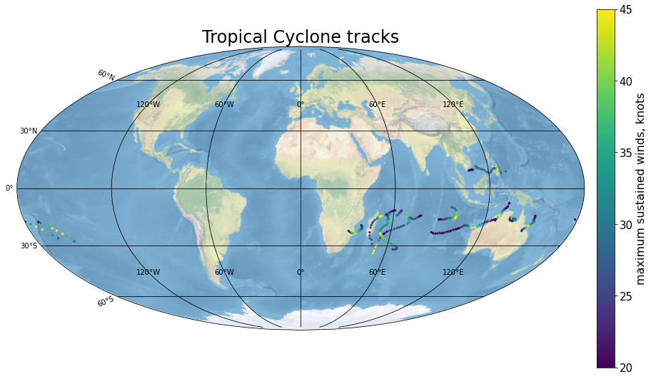
Caption: The figure generated shows Southern Hemisphere TC tracks for the selected time window. Each dot along the track shows the storm’s position at a given time. The color of each position shows the maximum sustained winds in knots.
Q4. Based on the map above, Are there many tropical cyclones in the South Atlantic ocean for the selected time window? Why? See: https://www.aoml.noaa.gov/hrd-faq/#south-atlantic-and-tcs.
insert Q4 answer here.
Based on your answer to Q3 define a time window for which to download TC data in the Northern Hemisphere:
#User inputs:
#format: 'yyyy-mm-dd'
#Disclaimer: time windows longer than 3 months may results in data query errors.
start = '2017-07-01'
end = '2017-10-30'
TCs = TC_and_storms_view(startDate=start,endDate=end,tag_TC_or_SH_FILT='TC') #startDate='2018-07-15',endDate='2018-09-15')
https://argovis.colorado.edu/tc/findByDateRange?startDate=2017-07-01T00:00:00&endDate=2017-10-30T00:00:00
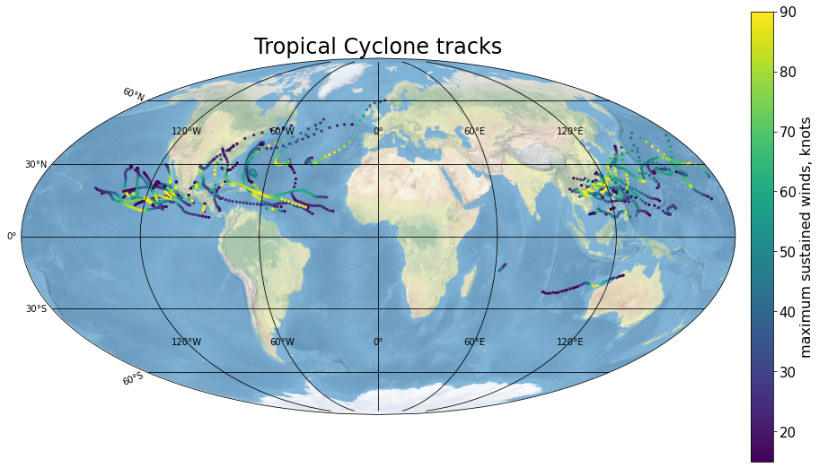
Caption: The figure generated shows Northern Hemisphere TC tracks for the selected time window. Each dot along the track shows the storm’s position at a given time. The color of each position shows the maximum sustained winds in knots.
Co-locating Argo profiles along TC track
Print a list of named tropical cyclones included in the map above for the Northern Hemisphere:
for x in TCs:
    if 'name' in x.keys():
        print('ID: ' + x['_id']+'; '+x['name']+' '+str(x['year']))
ID: AL182017_HURDAT2; PHILIPPE 2017
ID: EP202017_HURDAT2; SELMA 2017
ID: AL172017_HURDAT2; OPHELIA 2017
ID: AL162017_HURDAT2; NATE 2017
ID: EP192017_HURDAT2; RAMON 2017
ID: AL152017_HURDAT2; MARIA 2017
ID: AL142017_HURDAT2; LEE 2017
ID: EP182017_HURDAT2; PILAR 2017
ID: AL122017_HURDAT2; JOSE 2017
ID: EP172017_HURDAT2; NORMA 2017
ID: EP152017_HURDAT2; OTIS 2017
ID: EP162017_HURDAT2; MAX 2017
ID: AL112017_HURDAT2; IRMA 2017
ID: AL132017_HURDAT2; KATIA 2017
ID: EP142017_HURDAT2; LIDIA 2017
ID: AL092017_HURDAT2; HARVEY 2017
ID: EP132017_HURDAT2; KENNETH 2017
ID: AL082017_HURDAT2; GERT 2017
ID: EP122017_HURDAT2; JOVA 2017
ID: AL072017_HURDAT2; FRANKLIN 2017
ID: EP112017_HURDAT2; ELEVEN 2017
ID: EP102017_HURDAT2; IRWIN 2017
ID: AL062017_HURDAT2; EMILY 2017
ID: EP092017_HURDAT2; HILARY 2017
ID: EP072017_HURDAT2; GREG 2017
ID: EP062017_HURDAT2; FERNANDA 2017
ID: EP082017_HURDAT2; EIGHT 2017
ID: AL052017_HURDAT2; DON 2017
ID: EP052017_HURDAT2; EUGENE 2017
ID: AL042017_HURDAT2; FOUR 2017
ID: EP042017_HURDAT2; DORA 2017
Select a storm from the list above (name and year):
#User inputs:
tc_name = 'maria'#all lowercase
tc_year = 2017
Load the track for the storm of interest:
tc_star = get_TCs_byNameYear(tc_name,tc_year)
df  = pd.DataFrame(tc_star[0]['traj_data'])
https://argovis.colorado.edu/tc/findByNameYear?name=maria&year=2017
Set parameters for the co-location of Argo float profiles:
Here we set the temporal and spatial range for the co-location of Argo floats with the TC track of interest. The suggested parameters are: delta_days = 7 (days), dx = .75 (of a degree longitude), and dy = .75 (of a degree latitude), i.e. Argo profiles within a .75 degree box and a 7*2+1=15 days window (centered around each point on the TC track) will be considered. However, the user may change these if desired. The larger the temporal and spatial ranges, the more profiles will be included. Yet profiles may be further away from the TC in space and time and further apart from each other. This makes it more challenging to interpret the difference between the “before” versus “after” profile, as other factors (not associated with the TC) may play a role.
#User inputs:
#max number of days before and after TC passage to get profile pairs:
delta_days = 7
dx = .75 #degrees longitude
dy = .75 #degree latitude
presRange=[0,100] #decibar, [dbar] to plot profile. Larger range results in longer processing time
Co-locate Argo profiles along TC track and map location of profiles and TC track:
df                           = get_track_for_storm(tc_name,tc_year)
[prof_beforeTC,prof_afterTC] = map_TC_and_Argo(df, delta_days=delta_days, dx=dx, dy=dy, presRange=presRange,printing=True, printing_flag=df['_id'][0])
https://argovis.colorado.edu/tc/findByNameYear?name=maria&year=2017
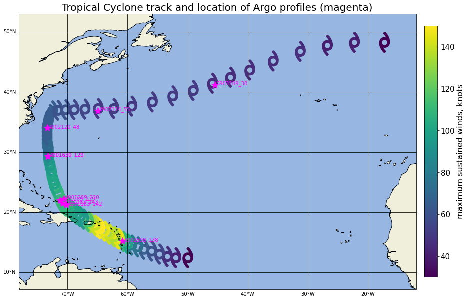
Caption: The figure generated here shows a map of the selected TC track. As before, each storm symbol shows the position of the storm and the color shows the TC’s maximum sustained winds in knots. Magenta stars show the position of Argo profiles co-located with the TC track.
Q5. Before we generate plots of before and after temperature and salinity profiles along the track: What do you expect will happen to ocean temperature and salinity after the passage of a Tropical Cyclone? Hint: see overall ‘Results’ section (Section 1.5) and reference therein, e.g. Zhang et al. (2021).
insert Q5 answer here.
Q6. What is (are) the physical mechanism(s) leading to these changes?
insert Q6 answer here.
Print ID (i.e. platformNumber_cycleNumber) of oceanic profiles that are co-located with the tropical cyclone of interest and make a profile plot:
This is done only for locations along the tropical cyclone track of interest (as defined above) where co-located oceanic profiles are available both before and after the cyclone.
print('>>>>>>>>> '+ tc_name+' '+str(tc_year)+' <<<<<<<<<')
plot_prof_pairs(prof_beforeTC,prof_afterTC,presRange)
>>>>>>>>> maria 2017 <<<<<<<<<
-------------
Temperature, before (black): 4901289_229
Temperature, after (red): 4901289_230
Salinity, before (black): 4901289_229
Salinity, after (red): 4901289_230
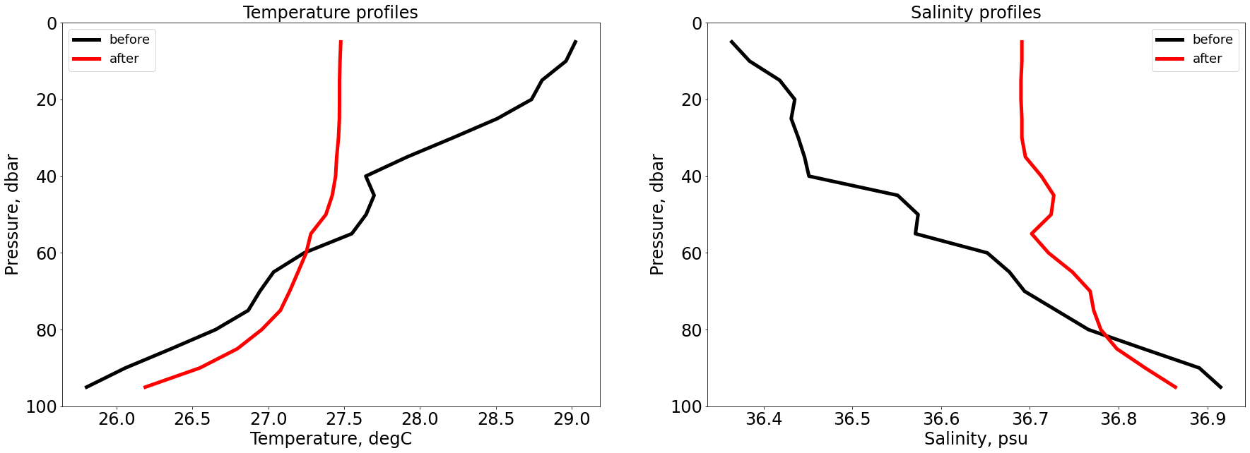
Caption: A figure is generated for each point of the tropical cyclone track of interest (as defined above) where co-located oceanic profiles are available both before and after the cyclone. Temperature profiles are on the left, salinity profiles are on the right: black profiles are measured before the TC passage, red profiles are measured after the TC passage. The x-axis of each panel shows the variable of interest (temperature or salinity), and the y-axis shows the pressure level.
Q7. Estimate the change in temperature and salinity before and after the tropical cyclone’s passage at different pressure levels. Where do you see the largest change?
insert Q7 answer here.
Q8. Let’s define the ocean heat content per unit area as: \(\partial{(OHC)} = \partial{T} \times \rho \times C_p \times \partial{z}\), where \(\partial{(OHC)}\) is the change in temperature in a layer of depth \(\partial{z}\), and we take the density, \(\rho = 1025\frac{kg}{m^3}\) and the specific heat, \(C_p = 3850 \frac{J}{kg \cdot C}\). Is there any change in the ocean heat content before and after the passage of the Tropical Cyclone? Estimate dOHC between the surface and 30 dbar, using dT at the shallowest pressure observed. Hint: for the purpose of this question dz can be approximated by dp, where p is pressure.
insert Q8 answer here.
Q9. Repeat the analysis for two more Tropical Cyclones, one in the same ocean basin, the other in a different ocean basin. Are the results consistent across Tropical Cyclones? Whether your analysis shows consistent results or not, should the results (i.e. the changes in temperature and salinity) be consistent across Tropical Cyclones? Why?
insert Q9 answer here.
Activity Results
Present your results. You should leverage the information and references provided through the notebook (Sections 1.5 and 4). Make direct reference to the figures you generated throughout the activity. Use your answers to the different questions throughout the activity to guide your results narrative.
insert your results here
Activity 2: Changes in oceanic properties as sea ice forms
The second activity in this notebook will guide users to explore sea-ice coverage estimates from SOSE and examine how ocean properties (as observed by Argo floats) change as sea-ice forms. For this, we will leverage the Argo float position QC flag: QC flag = 8, indicates that the position of the float is estimated. This may happen when the float does not surface because it is trapped under ice (hence it may serve as a proxy for sea-ice cover). The user will be able to select any particular date to examine. A map showing SOSE sea-ice estimate and location of Argo floats will be generated. A list of floats with estimated positions (i.e. thought to be under ice) will be printed on screen. The user will then generate a plot of the location and position QC flag for a float of interest (e.g. from the list) in order to identify when the float was thought to be under sea-ice. Finally, the user will generate a multi-panel plot showing: a) the time series of the float’s position QC flag value and fraction of sea-ice from SOSE, b) ocean temperature profiles in time as recorded by the float, and c) ocean salinity profiles in time as recorded by the float. SOSE sea-ice fraction is 0 if there is no ice over a given grid point, it is 1 if the area corresponding to a given grid point is covered by sea-ice.
Learning goals:
1- Use Argovis and Python to query Argo float and SOSE datasets, parse them, and generate plots.
2- Describe ocean temperature and salinity changes as sea-ice forms and melts.
3- Work collaboratively with your team to answer questions throughout the activity.
Q10. What is SOSE and what type of data does it leverage for its sea-ice estimates? (see: http://sose.ucsd.edu/sose.html)
insert Q10 answer here.
Q11. Does SOSE include Argo float observations? If so, do you expect the SOSE sea-ice estimates to be consistent with Argo floats observations?
insert Q11 answer here.
Data processing and analysis
Mapping SOSE sea-ice and Argo profile locations
Here the user will define the first set of parameters to begin the second activity. However, the user will define additional parameters as they advance through the activity.
Define region and date of interest for sea ice data:
Selected data will be shown on a map, based on which longitude and latitude ranges are defined in xreg_ALL and yreg_ALL and on what date is indicated in date_ALL (see example for the required format). xreg_ALL and yreg_ALL are lists defining longitude and latitude ranges in the overall region of interest: this is needed as there is a limit to the size of data that can be queried at the same time using the Argovis API. Hence, the map is populated one subregion at a time. Please note that the larger the region of interest, the longer the code will take to run, due to the high-resolution of SOSE sea-ice data. We have predefined a region that does not take too long to run, the user is welcome to explore other regions of different sizes.
#User inputs:
date_ALL = ['2013-06-01']
yreg_ALL = np.arange(-90.,-10.,40.).tolist()
xreg_ALL = np.arange(-60.,-30.,5.).tolist()
Define the co-location strategy for sea ice and Argo profiles, i.e. how many days before and after the sea ice field we query profiles for:
If delta_argo=3, a 7 day window (centered on the date selected for the sea-ice map of interest) is used.
#User defined:
delta_argo = 3
#The user may change the first two parameters below if desired, but it is not required:
presRange='[0,50]' # pressure range of interest for Argo profiles
plev_presRange = 30 # a number in the middle of the pressure range of interest should work for this
color_map = plt.cm.get_cmap('Blues')
Map sea-ice field and location of co-located Argo profiles (marked based on their position QC flag):
Argo position QC flag legend: - 0: no quality control performed - 1: good data (‘+’ symbol in map) - 2: probably good data - 3: probably bad data - 4: bad data - 5: value changed - 6: n/a - 7: n/a - 8: position estimated (‘o’ symbol in map) - 9: missing value - ‘’: Fill value
SeaIce_Argo = map_seaice_argo(date_ALL,yreg_ALL,xreg_ALL,delta_argo,presRange,plev_presRange,color_map)
>>>> Profile ID for profiles under ice (i.e. platformNumber_profileNumber) <<<<
0    7900408_18
0    7900401_18
Name: profile_id, dtype: object
0    7900412_18
0    7900414_18
Name: profile_id, dtype: object
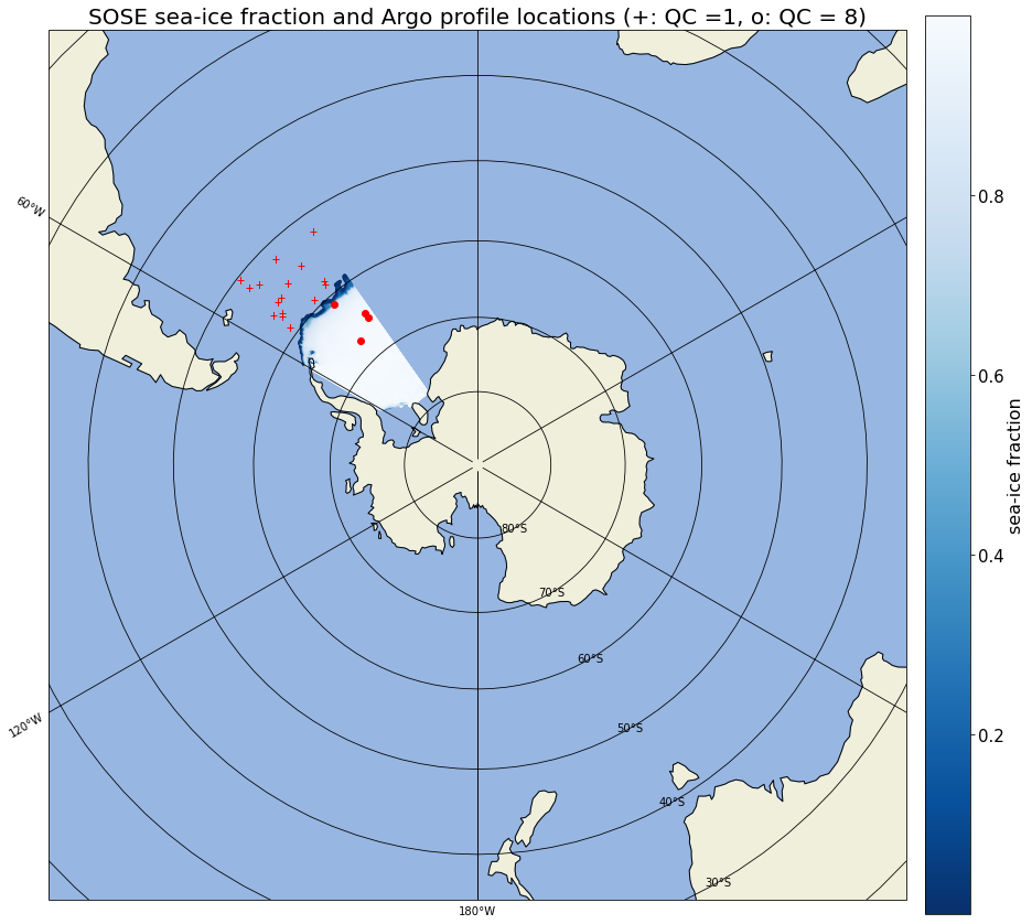
Caption: The figure generated shows a map of the sea-ice field for the date and region defined above. In addition, the location of co-located Argo profiles is plotted with red markers: dots show profiles with position QC = 8, crosses show profiles with position QC=1. A list of profile IDs is printed on screen for co-located profiles with position QC = 8
Q12. According to the map, do you see a good general agreement between SOSE sea-ice coverage and Argo profiles that have position QC = 8 (position estimated)? Remember that when the position is estimated, the float has not surfaced and, at high latitudes, it is likely to be trapped under sea-ice.
insert Q12 answer here.
Q13. Is there a region in general where there is disagreement between the model and Argo? (i.e. model indicates sea-ice coverage but Argo profiles have position QC = 1 (good position information), or model indicates no sea-ice and Argo profiles have position QC=8 (position estimated))
insert Q13 answer here.
Q14. SOSE leverages observations including Argo profiles (see Q12): even if you indicated no disagreement in your answer to Q13, could there be disagreement in other regions and/or days? Why?
insert Q14 answer here.
Mapping Argo float locations and position QC flag history
Select a float from the list above:
#User defined:
platform_number = '7900414'
Query profiles measured by the float selected:
In the following, we query profiles for the float of interest and Interpolate them on selected pressure levels (defined in plevIntp). Information available for the float will be printed on the screen.
platformProfiles = get_platform_profiles(platform_number) #'3900737')#('5904684')
# platformDf = parse_into_df(platformProfiles)
# print('number of measurements {}'.format(platformDf.shape[0]))
plevIntp = np.arange(5,505,5)
platformDf_plev = parse_into_df_plev(platformProfiles, plevIntp)
platformDf_plev.head()
temp2d = np.concatenate(platformDf_plev['temp'].to_numpy()).ravel().reshape(len(platformDf_plev['temp']),len(plevIntp)).T
psal2d = np.concatenate(platformDf_plev['psal'].to_numpy()).ravel().reshape(len(platformDf_plev['temp']),len(plevIntp)).T
Index(['bgcMeasKeys', 'station_parameters', 'station_parameters_in_nc',
       'PARAMETER_DATA_MODE', '_id', 'POSITIONING_SYSTEM', 'DATA_CENTRE',
       'PI_NAME', 'WMO_INST_TYPE', 'DATA_MODE', 'PLATFORM_TYPE',
       'measurements', 'pres_max_for_TEMP', 'pres_min_for_TEMP',
       'pres_max_for_PSAL', 'pres_min_for_PSAL', 'max_pres', 'date',
       'date_added', 'date_qc', 'lat', 'lon', 'geoLocation', 'position_qc',
       'cycle_number', 'dac', 'platform_number', 'nc_url', 'DIRECTION',
       'BASIN', 'url', 'core_data_mode', 'jcommopsPlatform',
       'euroargoPlatform', 'formatted_station_parameters', 'roundLat',
       'roundLon', 'strLat', 'strLon', 'date_formatted', 'id', 'temp', 'psal',
       'pres'],
      dtype='object')
Plot profile locations for the float of interest, color coded by the position QC flag at each location:
Argo position QC flag legend: - 0: no quality control performed - 1: good data - 2: probably good data - 3: probably bad data - 4: bad data - 5: value changed - 6: n/a - 7: n/a - 8: position estimated - 9: missing value - ‘’: Fill value
QC_location_plot = plot_argo_QC_location(platform_number,platformDf_plev['lon'],platformDf_plev['lat'],platformDf_plev['position_qc'])
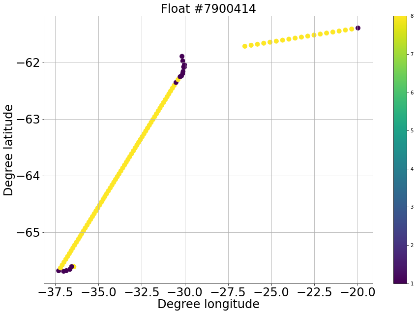
Caption: The figure shows where the selected Argo float measured profiles. The color of each dot indicates the position QC flag for each profile.
Q15. Why do some profile locations (for the float of interest) follow a straight line? Note this happens when the position QC = 8.
insert Q14 answer here.
For the Argo float of interest, plot temperature, salinity and position QC flag history, along with co-located sea-ice fraction from SOSE
Download and save sea-ice fraction from SOSE:
dx = 1/6 # based on SOSE resolution
dy = 1/6 # based on SOSE resolution
# 2013-06-01
# <class 'str'>
seaice_val = []
for (ilon,ilat,idate) in zip(tqdm(platformDf_plev['lon']),platformDf_plev['lat'],platformDf_plev['date']):
    time.sleep(0.01)
    try:
        bfr  = get_SOSE_sea_ice(xreg=[ilon-dx,ilon+dx],yreg=[ilat-dy,ilat+dy],date=idate[0:10],printUrl=False)
        bfr_df_SeaIce       = parse_into_df_SeaIce(bfr)
        #         print(ilon,ilat)
        #         print(bfr_df_SeaIce)
        seaice_val.append(interpolate.griddata((bfr_df_SeaIce['lon'],bfr_df_SeaIce['lat']),bfr_df_SeaIce['value'],(ilon,ilat)))
        #break
        #df = pd.concat([df, bfrDf], sort=False)
        #find point closest to target (will not try and interpolate)
    except:
        seaice_val.append(np.array(0))
        pass
Define maximum number of days permitted between profiles from the float of interest:
In the case there are no profiles within the maximum number of days allowed, we include an empty profile in the float history. This is done to avoid interpolation of the data over a period longer than tdelta in the upcoming contour plot.
#User defined:
tdelta = 15
After adding empty profiles to the float history as needed, we will generate a multi-panel figure showing: a) the time series of the float’s position QC flag value and co-located fraction of sea-ice from SOSE, b) ocean temperature profiles in time as recorded by the float and, c) ocean salinity profiles in time as recorded by the float:
time_series = plot_SeaIce_argo_QC_temp_sal(plevIntp,temp2d,psal2d,platformDf_plev,tdelta,seaice_val,platform_number)
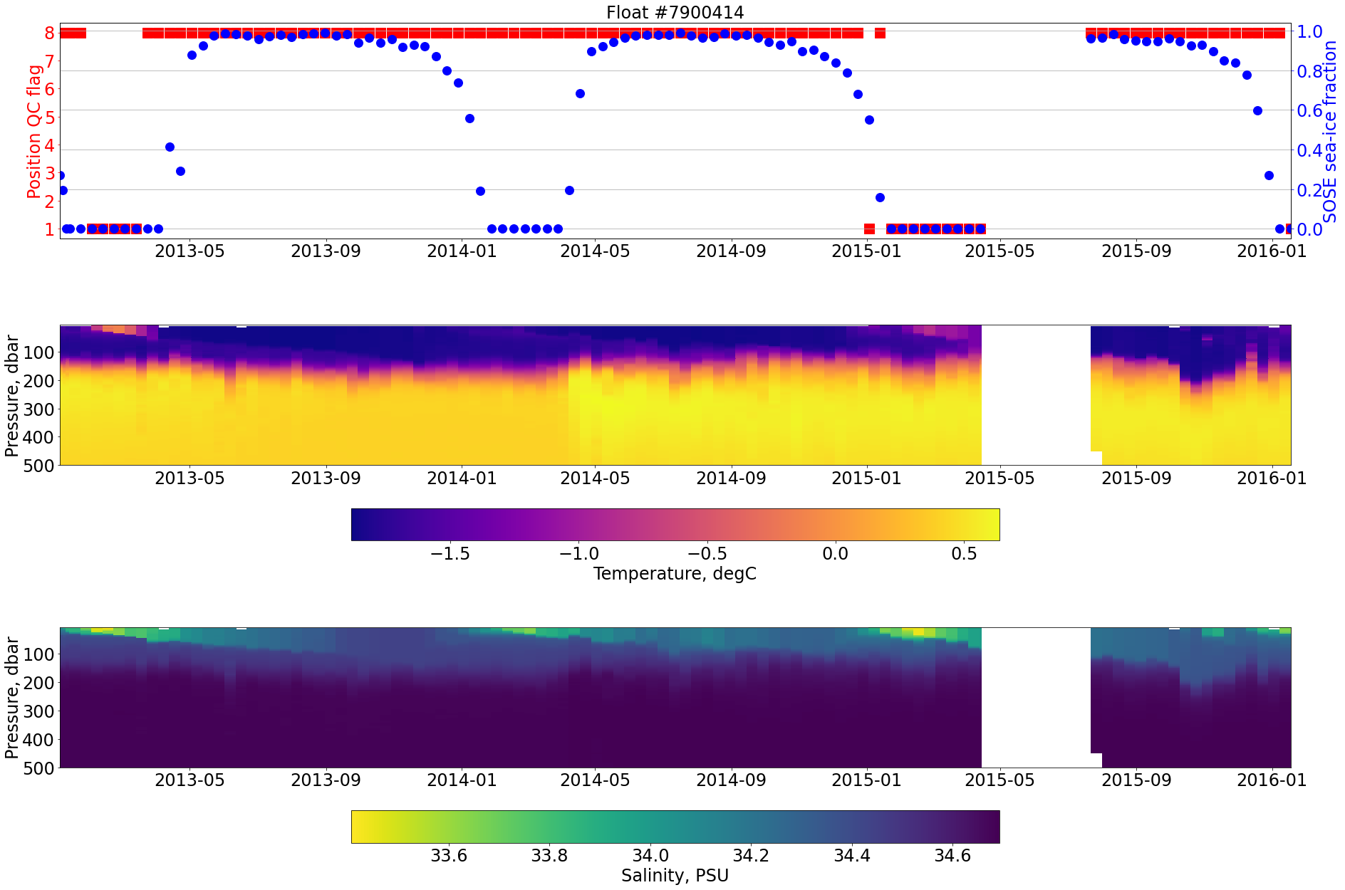
Caption: The top panels shows a time series of the float position QC flag (red) and SOSE sea-ice fraction (blue) for each position of the float.The middle panel shows a Hovmoller diagram of temperature (color) in depth (pressure, y-axis) and time (x-axis).The bottom panel shows a Hovmuller diagram of salinity (color) in depth (pressure, y-axis) and time (x-axis).
Q16. How do ocean temperature and salinity change after sea-ice formation? What is(are) the physical mechanism(s) leading to these changes? Hint: see overall ‘Results’ section (Section 1.5) and references there in. E.g. National Snow and Ice Data Center.
insert Q15 answer here.
Q17. Describe changes to the mixed layer as sea-ice forms and melts. Hint: see overall ‘Results’ section (Section 1.5) and references there in. E.g. Pellichero et al. (2016).
insert Q16 answer here.
Activity Results
Present your results. You should leverage the information and references provided throughout the notebook (Sections 1.5 and 5). Make direct reference to the figures you generated throughout the activity. Use your answers to the different questions throughout the activity to guide your results narrative.
insert results text here
References
Argo (2000). Argo float data and metadata from Global Data Assembly Centre (Argo GDAC). SEANOE. doi:10.17882/42182.
A. Verdy and M. Mazloff, 2017: A data assimilating model for estimating Southern Ocean biogeochemistry. J. Geophys. Res. Oceans., 122, doi:10.1002/2016JC012650.
Frew, R. C., Feltham, D. L., Holland, P. R., & Petty, A. A. (2019). Sea Ice–Ocean Feedbacks in the Antarctic Shelf Seas, Journal of Physical Oceanography, 49(9), 2423-2446. doi:10.1175/JPO-D-18-0229.1
M. Mazloff, P. Heimbach, and C. Wunsch, 2010: An Eddy-Permitting Southern Ocean State Estimate. J. Phys. Oceanogr., 40, 880-899. doi:10.1175/2009JPO4236.1..
Pellichero, V., Sallée, J.-B., Schmidtko, S., Roquet, F., and Charrassin, J.-B. (2017), The ocean mixed layer under Southern Ocean sea‐ice: Seasonal cycle and forcing, J. Geophys. Res. Oceans, 122, 1608– 1633, doi:10.1002/2016JC011970.
Priestley, M. D. K., Ackerley, D., Catto, J. L., Hodges, K. I., McDonald, R. E., & Lee, R. W. (2020). An Overview of the Extratropical Storm Tracks in CMIP6 Historical Simulations, Journal of Climate, 33(15), 6315-6343. doi:10.1175/JCLI-D-19-0928.1.
Tucker, T., Giglio, D., and Scanderbeg, M. (2020). Argovis API exposed in a Python Jupyter notebook: an easy access to Argo profiles, weather events, and gridded products. Earth and Space Science Open Archive, doi:10.1002/essoar.10504304.1.
Tucker, T., Giglio, D., Scanderbeg, M., & Shen, S. S. P. (2020). Argovis: A Web Application for Fast Delivery, Visualization, and Analysis of Argo Data, Journal of Atmospheric and Oceanic Technology, 37(3), 401-416. doi:10.1175/JTECH-D-19-0041.1.
Zhang, H., He, H., Zhang, WZ. et al. Upper ocean response to tropical cyclones: a review. Geosci. Lett. 8, 1 (2021). doi:10.1186/s40562-020-00170-8.