BC_01 Bias Corrected Estimation of Paleointensity
Table of Contents
Author(s)
Author1={"name":"Brendan Cych","affiliation":"Scripps Institution of Oceanography, UCSD","email":"bcych@ucsd.edu","orcid":"0000-0003-2387-3544"}
Author2={"name":"Matthias Morzfeld","affiliation":"Scripps Institution of Oceanography, UCSD","email":"matti@ucsd.edu","orcid":"0000-0003-2257-8930"}
Author3={"name":"Lisa Tauxe","affiliation":"Scripps Institution of Oceanography, UCSD","email":"ltauxe@ucsd.edu","orcid":"0000-0002-4837-8200"}
Purpose
Paleointensities are estimates of the Earth’s ancient magnetic field strength, obtained from materials including rocks and pottery sherds which cooled in that field. Paleointensity can be obtained by comparing the magnetization lost on cooling a specimen in zero field, to the magnetization gained on cooling in a known lab field. The theoretical relationship between these two magnetizations should be proportional at all temperatures for an ideal specimen, with the ratio of magnetization lost/magnetization gained being the same as the ratio of ancient field/lab field.
In natural samples, the assumptions of the paleointensity experiment are frequently violated, leading to non linear behaviour on the Arai plot (Nagata et al, 1963). Traditionally, paleomagnetists use “selection criteria” to exclude specimens from the analysis if they believe they violate the experimental assumptions. These criteria are generally based on an empirical description of non-ideal behaviour, with a specimen being excluded if it fails to meet a threshold value. There is little agreement between labs on which set of criteria to use.
Bias Corrected Estimation of Paleointensity (BiCEP) is a new method for analyzing Thellier-type paleointensity data. Instead of excluding specimens from the analysis, BiCEP assumes that the paleointensity estimate for each specimen has some amount of bias based on the values of the curvature criterion of Paterson (2011). In this way we can estimate the unbiased value of the paleointensity.
BiCEP differs from other methods of paleointensity analysis, because it reduces the number of experiments that need to be excluded from the analysis. The credible intervals produced by BiCEP are more reliable than the standard deviation traditional selection criteria, with the precision on the estimate starting low, and increasing as more specimens are measured. It also allows for weighting of results from different specimens, as better results contribute more to the estimate than worse results. BiCEP can be used to analyze new paleointensity data, and to reanalyze old paleointensity data using a consistent methodology which significantly reduces the number of subjective choices needed to make a paleointensity estimate.
Technical contributions
This notebook
Uses the BiCEP_functions library to read in, plot and analyze paleointensity data.
Uses a Markov Chain Monte Carlo (MCMC) sampler using the
pystanpackage (http://mc-stan.org) to determine the relationship between the curvature (\(\vec{k}\)) parameter (Paterson, 2011) for specimens which were magnetized in the same field.Allows you to save these data into the MagIC database format (https://www2.earthref.org/MagIC)
Demonstrates a GUI which allows you to perform the previous steps more easily.
Methodology
Thellier Type Paleointensity data must be imported using the MagIC format. A measurements.txt, specimens.txt, samples.txt and sites.txt are required. These are then saved as an internal csv format for use with BiCEP.
Paleointensity data can be plotted and some limited analysis using different selection criteria can be performed.
The BiCEP method can be fit to a collection of specimens, either sample or site, and the results can be plotted. Reanalysis is possible. For more information on the paleointensity method- see the citation for more detailed information on how the method operates.
The results of the BiCEP method can be saved to MagIC format.
Results
The BiCEP method yields a similar number of accurate paleointensity estimates to the looser sets of traditional selection criteria analyzed, but with higher precision and accuracy more akin to tighter sets of criteria which yield fewer estimates. See Figure 7 in Cych et al (in press) for more information.
Funding
Award1 = {"agency": "National Science Foundation", "award_code": "EAR1547263", "award_URL": "award_URL"}
Award2 = {"agency": "National Science Foundation", "award_code": "EAR1827263", "award_URL": "award_URL"}
Keywords
Include up to 5 keywords, using the template below.
keywords=[“Data Analysis”, “Paleomagnetism”, “Paleointensity”, “Markov Chain Monte Carlo”, “Bayesian Statistics”]
Citation
Cych et al (In Press) doi: 10.1002/essoar.10506403.1 https://www.essoar.org/doi/10.1002/essoar.10506403.1
Acknowledgements
We are deeply grateful to Lennart de Groot and Greig Paterson for their very helpful reviews and for the advice and guidance given by Andrew Roberts, David Heslop and Joseph Wilson.
Setup
Library import
import pandas as pd
import matplotlib.pyplot as plt
%matplotlib inline
from IPython.display import Image
Local library import
import sys
sys.path.append('modules_and_scripts/')
#The BiCEP_functions library imports all other needed libraries
import BiCEP_functions as BiCEP
Parameter definitions
B_exp=36.4 #The expected field for the site we will be using BiCEP with today
Data import
We can produce a data file that BiCEP can read internally from the magic format using the generate_arai_plot_table function in BiCEP_GUI. We will specify an output name of example_data.csv. For your convenience, we have included a set of MagIC formatted data to convert to the BiCEP format. This may take a few minutes
BiCEP.generate_arai_plot_table('example_data')
INFO:numexpr.utils:NumExpr defaulting to 8 threads.
-I- Using online data model
-I- Getting method codes from earthref.org
-I- Importing controlled vocabularies from https://earthref.org
Working on: AL2360-1a
Working on: AL2360-1b
Working on: AL2360-1c
Working on: AL2360-1d
Working on: AL2360-1e
Working on: AL2742-4a
Working on: AL2742-4b
Working on: AL2742-4e
Working on: AL2742-4f
Working on: AL2742-4g
Working on: AL2770-3a
Working on: AL2770-3b
Working on: AL2770-3c
Working on: AL2844-2a
Working on: AL2844-2b
Working on: AL2852-2a
Working on: AL2852-2b
Working on: AL2852-2c
Working on: AL2852-2d
Working on: AL2852-2e
Working on: AL2852-2f
Working on: AL3023-1a
Working on: AL3023-1b
Working on: AL3028-2a
Working on: AL3028-2b
Working on: AL3029-4a
Working on: AL3029-4b
Working on: AL3029-4c
Working on: AL3029-5a
Working on: AL3031-1a
Working on: AL3031-1b
Working on: AL3031-1c
Working on: AL3031-1d
Working on: AL3034-2a
Working on: AL3034-2d
Working on: AL3034-2e
Working on: AL3034-5a
Working on: AL3034-5b
Working on: AL3034-5d
Working on: AL3035-2a
Working on: AL3035-2b
Working on: AL3035-2h
Working on: AL3035-2i
Working on: AL3035-2j
Working on: AL3156-1a
Working on: AL3156-1b
Working on: AL3159-1a
Working on: AL3159-1b
Working on: AL3159-1g
Working on: AL3166-1a
Working on: AL3166-1b
Working on: AL3166-1g
Working on: AL3166-1h
Working on: hw108a1
Working on: hw108a2
Working on: hw108a3
Working on: hw108a4
Working on: hw108a5
Working on: hw108b1
Working on: hw108b2
Working on: hw108b3
Working on: hw108b4
Working on: hw108b5
Working on: hw108c1
Working on: hw108c2
Working on: hw108c3
Working on: hw108c4
Working on: hw108c5
Working on: hw123a1
Working on: hw123a2
Working on: hw123a3
Working on: hw123a4
Working on: hw123a5
Working on: hw126a1
Working on: hw126a2
Working on: hw126a3
Working on: hw126a4
Working on: hw126a5
Working on: hw126b1
Working on: hw126b2
Working on: hw126b3
Working on: hw126b4
Working on: hw126b5
Working on: hw128a1
Working on: hw128a2
Working on: hw128a3
Working on: hw128a4
Working on: hw128a5
Working on: hw128b1
Working on: hw128b2
Working on: hw128b3
Working on: hw128b4
Working on: hw128b5
Working on: hw128c1
Working on: hw128c2
Working on: hw128c3
Working on: hw128c4
Working on: hw128c5
Working on: hw128d1
Working on: hw128d2
Working on: hw128d3
Working on: hw128d4
Working on: hw128d5
Working on: hw108c10
Working on: hw108c11
Working on: hw108c12
Working on: hw108c13
Working on: hw108c6
Working on: hw108c7
Working on: hw108c8
Working on: hw108c9
Working on: hw123a10
Working on: hw123a11
Working on: hw123a12
Working on: hw123a6
Working on: hw123a7
Working on: hw123a8
Working on: hw123a9
Working on: hw126a6
Working on: hw126a7
Working on: hw126a8
Working on: hw128a10
Working on: hw128a11
Working on: hw128a6
Working on: hw128a7
Working on: hw128a8
Working on: hw128a9
Working on: hw201a1
Working on: hw201a10
Working on: hw201a11
Working on: hw201a12
Working on: hw201a2
Working on: hw201a3
Working on: hw201a4
Working on: hw201a5
Working on: hw201a6
Working on: hw201a7
Working on: hw201a8
Working on: hw201a9
Working on: hw226a1
Working on: hw226a2
Working on: hw226a3
Working on: hw226a4
Working on: hw226a5
Working on: hw226a6
Working on: hw226b1
hw226b1 in site hw226 Not included, demagnetization not completed
Working on: hw226b2
Working on: hw226b3
Working on: hw226b4
Working on: hw226b5
Working on: hw226b6
Working on: hw241a1
Working on: hw241a2
Working on: hw241a3
Working on: hw241a4
Working on: hw241a5
Working on: hw241a6
Working on: hw241d1
Working on: hw241d2
Working on: hw241d3
Working on: hw241d4
Working on: hw241d5
Working on: hw241d6
Working on: hw241e1
Working on: hw241e2
Working on: hw241e3
Working on: hw241e4
Working on: hw241e5
Working on: hw241e6
Working on: BR06-3F
Working on: BR06-4F
Working on: BR06-5F
Working on: p1ay
Working on: p1c-stub1
Working on: p1cy_u
Working on: p1cz_u
Working on: p1e_u
Working on: p1fx_u
Working on: p1fy_u
Working on: p1ga_u
Working on: p1gb_u
Working on: p1gc_u
Working on: p1h_u
Working on: p1hb_u
Working on: p1ka_u
Working on: p1kb_u
Working on: p1kc_u
Working on: p1kd_u
Working on: p1l_u
Working on: p1my
Working on: p1na_u
Working on: p1nb
Working on: p1o_u
Working on: p2aa_u
Working on: p2ab_u
Working on: p2ac_u
Working on: p2ad
Working on: p2b_u
Working on: p2d
Working on: p2ey_u
Working on: p2kx_u
Working on: p2na_u
Working on: p2nb_u
Working on: p2o_u
Working on: p2q
Working on: p2qc
Working on: p2rl_u
Working on: p2s_u
Working on: vm1a
Working on: vm1c
Working on: vm1dy
Working on: vm1f
Working on: vm1g
Working on: vm1hx
Working on: vm1i
Working on: vm1kx
Working on: vm1mx
Working on: vm1my
Working on: vm1nx
Working on: vm1o
Working on: vm1q
Working on: vm1ry
Working on: vm1s
Working on: vm2ay
Working on: vm2by
Working on: vm2dy
Working on: SBG_2352-2b
Working on: SBG_2352-2e
Working on: SBG_2352-2g
Working on: SBG_2358-4f
Working on: SBG_2372-2e
Working on: SBG_2372-2g
Working on: SBG_2372-2h
Working on: SBG_2372-3d
Working on: SBG_2372-3e
Working on: SBG_2372-3f
Working on: SBG_2392-4c
Working on: SBG_2392-4e
Working on: rs25b
Working on: rs25e
Working on: rs26c
Working on: rs27a
Working on: rs27d
Working on: rs25a
Working on: rs25c
Working on: rs25d
Working on: rs26a
Working on: rs26b
Working on: rs26d
Working on: rs26e
Working on: rs27b
Working on: rs27c
Working on: rs27e
Working on: rs27f
Working on: rs27g
Working on: rs27h
Working on: rs27i
Working on: rs27j
Working on: remag-rs61a
Working on: remag-rs61c
Working on: remag-rs61e
Working on: remag-rs61f
Working on: remag-rs61h
Working on: remag-rs61i
Working on: remag-rs62a
Working on: remag-rs62b
Working on: remag-rs62e
Working on: remag-rs62f
Working on: remag-rs62g
Working on: remag-rs62h
Working on: remag-rs63a
Working on: remag-rs63f
Working on: remag-rs63g
Working on: remag-rs63i
Working on: remag-rs63j
Working on: remag-rs78a
Working on: remag-rs78e
Working on: remag-rs78f
Working on: remag-rs78g
remag-rs78g in site remag-rs78 Not included, demagnetization not completed
Working on: remag-rs78i
Working on: kf011
Working on: kf031
Working on: kf072
Working on: A-1-3
Working on: A-2-3
Working on: A-3-3
Working on: A-4-3
Working on: A-4-4L
Working on: A-5-3
Working on: B-1-3
Working on: B-10-1
Working on: B-2-1
Working on: B-3-3
Working on: B-4-3
Working on: B-5-1
Working on: B-6-3
Working on: B-7-3
Working on: B-8-1
Working on: B-9-3
Working on: B-9-4L
Working on: C-1-3
Working on: C-2-3
Working on: C-3-3
Working on: C-4-1
Working on: C-4-4L
Working on: SW01-01A-2
Working on: SW01-02A-2
Working on: SW01-03A-2
Working on: SW01-04A-2
Working on: SW01-05A-2
Working on: SW01-06A-2
Working on: SW01-07A-2
Working on: SW01-08A-2
Working on: SW01-09A-2
Working on: SW01-10A-2
Working on: SW01-11A-2
Working on: SW01-12A-2
Working on: SW01-13A-2
Working on: SW01-14A-2
Working on: SW01-15A-2
Working on: SW01-16A-2
Working on: SW01-17A-2
Working on: SW01-18A-2
Working on: SW01-19A-2
Working on: TS01-00A-2
Working on: TS01-01A-2
Working on: TS01-02A-2
Working on: TS01-04A-1
Working on: TS01-05A-2
Working on: TS01-06A-3
Working on: TS01-07A-2
Working on: TS01-08A-2
Working on: TS01-10A-2
Working on: TS01-11A-2
Working on: TS01-12A-2
Working on: TS01-13A-2
Working on: TS01-14A-2
Working on: TS01-15A-2
Working on: TS01-16A-2
Working on: TS01-17A-2
Working on: TS01-18A-2
Working on: TS01-19A-2
Working on: TS01-20A-2
Working on: TS01-21A-2
Working on: TS01-22A-2
Working on: TS01-23A-2
Working on: TS01-24A-2
Working on: TS01-25A-2
Working on: TS01-26A-2
Working on: TS01-27A-2
Working on: TS01-28A-2
Working on: TS02-01A-2
Working on: TS02-02A-2
Working on: TS02-03A-2
Working on: TS02-04A-2
Working on: TS02-05A-3
Working on: TS02-06A-2
Working on: TS02-07A-2
Working on: TS02-08A-2
Working on: TS02-09A-3
Working on: TS02-10A-3
Working on: TS02-11A-2
Working on: TS02-12A-2
Working on: TS02-13A-2
Working on: TS02-14A-2
Working on: TS02-15A-2
Working on: TS02-16A-2
Working on: TS02-17A-2
Working on: TS02-18A-2
Working on: TS02-19A-2
Working on: TS02-20A-3
Working on: TS02-21A-2
Working on: TS02-22A-2
Working on: TS02-23A-2
Working on: TS02-24A-2
Working on: TS02-25A-2
Working on: TS02-26A-2
Working on: ET1_279BS
ET1_279BS in site ET1 Not included, demagnetization not completed
Working on: ET1_283E
ET1_283E in site ET1 Not included, demagnetization not completed
Working on: ET1_287D
Working on: ET1_289D
Working on: ET1_311E
Working on: ET1_318A
ET1_318A in site ET1 Not included, demagnetization not completed
Working on: ET2_182B
Working on: ET2_185A
ET2_185A in site ET2 Not included, demagnetization not completed
Working on: ET2_187A
ET2_187A in site ET2 Not included, demagnetization not completed
Working on: ET2_192A
ET2_192A in site ET2 Not included, demagnetization not completed
Working on: ET2_196D
Working on: ET3_008A
Working on: ET3_023E2
Working on: ET3_059C
Working on: ET3_064C
Working on: ET3_146A
ET3_146A in site ET3 Not included, demagnetization not completed
Working on: ET3_150B
ET3_150B in site ET3 Not included, demagnetization not completed
Working on: MGH1
Working on: W1
Working on: W2
Working on: W3
Working on: W4
Working on: W5
Working on: W6
Working on: LV10D3A
Working on: LV11A2
Working on: LV12A2A
Working on: LV12D1
Working on: LV12E2
Working on: LV14C3A
Working on: LV15B1
Working on: LV16A2B
Working on: LV16B1B
Working on: LV17A1A
Working on: LV18B3
Working on: LV19A2
Working on: LV19B1A
LV19B1A in site LV Not included, demagnetization not completed
Working on: LV19C1
Working on: LV19D3
Working on: LV19E1
Working on: LV19F2
Working on: LV19G2B
Working on: LV20B1
Working on: LV20C2
Working on: LV21A2
Working on: LV21B1
Working on: LV21C1
Working on: LV22D1
Working on: LV23A2
Working on: LV25C3
Working on: LV26D2
Working on: LV27B2
Working on: LV28E3A
Working on: LV29B2A
Working on: LV30A3A
Working on: LV30B2
Working on: LV30D1
Working on: LV3B3
Working on: LV4A3
Working on: LV4C3
Working on: LV6A2
Working on: LV6C3A
Working on: LV6D1B
Working on: LV6G1
Working on: LV6I3A
Working on: LV7B1
Working on: LV7G1
Working on: LV7H1
Working on: LV9A2
Working on: LV9F2
Working on: M3B5
Working on: M3C5
Working on: M3G2
M3G2 in site MSH Not included, demagnetization not completed
Working on: M3L1
M3L1 in site MSH Not included, demagnetization not completed
Working on: M3O6
Working on: M3S2
M3S2 in site MSH Not included, demagnetization not completed
Working on: M3U2
M3U2 in site MSH Not included, demagnetization not completed
Working on: M3V1
M3V1 in site MSH Not included, demagnetization not completed
Working on: M4F6
M4F6 in site MSH Not included, demagnetization not completed
Working on: M4G5
M4G5 in site MSH Not included, demagnetization not completed
Working on: M4M5
M4M5 in site MSH Not included, demagnetization not completed
Working on: M4S2
M4S2 in site MSH Not included, demagnetization not completed
Working on: M4T3
Working on: M4U1
M4U1 in site MSH Not included, demagnetization not completed
Working on: M4V1
M4V1 in site MSH Not included, demagnetization not completed
Working on: M5B2
M5B2 in site MSH Not included, demagnetization not completed
Working on: M5D1
Working on: M5E2
Working on: M5G1
M5G1 in site MSH Not included, demagnetization not completed
Working on: M5M2
M5M2 in site MSH Not included, demagnetization not completed
Working on: M5N2
M5N2 in site MSH Not included, demagnetization not completed
Working on: M5N5
Working on: M5P2
Working on: M5Q1
Working on: M5S2
Working on: M5T2
M5T2 in site MSH Not included, demagnetization not completed
Working on: M5W2
M5W2 in site MSH Not included, demagnetization not completed
Working on: M6B7A
Working on: M6C2
M6C2 in site MSH Not included, demagnetization not completed
Working on: M6D1
Working on: M6E13
Working on: M6G1
Working on: M6K1
Working on: M6L2
M6L2 in site MSH Not included, demagnetization not completed
Working on: M6M1
Working on: M6O3
Working on: M6P3
Working on: M6Q2
Working on: M6R4
M6R4 in site MSH Not included, demagnetization not completed
Working on: M6U2
M6U2 in site MSH Not included, demagnetization not completed
Working on: cr405g1-CZb
Working on: cr418f-CZb
Working on: cr423c-CZb
Working on: hw226a-SZb
Working on: jm009c1-CZb
Working on: jm009d1-CZb
Working on: jm009f2-CZb
Working on: jm009i2-CZb
Working on: jm011d1-CZb
Working on: mc109d-SZb
Working on: mc109e-SZb
Working on: mc111d-SZb
Working on: mc111e-SZb
Working on: mc117a-SZb
Working on: mc117b-SZb
Working on: mc117d-SZb
PTRM check at 373.0K has no corresponding infield measurement, ignoring
Working on: mc117e-SZb
Working on: mc120b-SZb
Working on: mc120c-SZb
Working on: mc167d2-SZb
Working on: sc02e1-CZb
Working on: sc03f-CZb
Working on: sc03h-CZb
Working on: sc06d-CZb
Couldn't find Anisotropy Tensors, Generating...
replacing existing ATRM data for  rs25a
replacing existing ATRM data for  rs25b
replacing existing ATRM data for  rs25c
replacing existing ATRM data for  rs25d
replacing existing ATRM data for  rs25e
replacing existing ATRM data for  rs26a
replacing existing ATRM data for  rs26b
replacing existing ATRM data for  rs26c
replacing existing ATRM data for  rs26d
replacing existing ATRM data for  rs26e
replacing existing ATRM data for  rs27a
replacing existing ATRM data for  rs27b
replacing existing ATRM data for  rs27c
replacing existing ATRM data for  rs27d
replacing existing ATRM data for  rs27e
566  records written to file  /home/brendan/BiCEP_GUI/specimens.txt
replacing existing AARM data for  hw108a1
replacing existing AARM data for  hw108c1
replacing existing AARM data for  hw108c10
replacing existing AARM data for  hw108c11
replacing existing AARM data for  hw123a1
replacing existing AARM data for  hw123a3
replacing existing AARM data for  hw123a4
replacing existing AARM data for  hw123a9
replacing existing AARM data for  hw126a4
replacing existing AARM data for  hw126a5
replacing existing AARM data for  hw241e2
replacing existing AARM data for  hw241e3
566  records written to file  /home/brendan/BiCEP_GUI/specimens.txt
-W- WARNING: Can't fit tanh function to NLT data for rs25b
When imported, BiCEP data is stored internally as a set of nested objects, one for the dataset which contains a object for each site (a set of samples expected to have been magnetized in the same field), or each sample (an object collected in the field) which are described using a SpecimenCollection object. Each of these SpecimenCollection objects contains an object for each specimen, which is a subsample that a set of independent measurements are made on. To make the data class, we can initialize a ThellierData object using our example_data.csv file. This may take a few seconds to create all of the objects. Printing our ThellierData object allows us to see the number of sites and specimens.
data=BiCEP.ThellierData('example_data.csv')
print(data)
Set of Thellier Data Containing the Sites:
1991-1992 Eruption Site	(53 specimens)
hw108	(23 specimens)
hw123	(12 specimens)
hw126	(13 specimens)
hw128	(26 specimens)
hw201	(12 specimens)
hw226	(11 specimens)
hw241	(18 specimens)
BR06	(3 specimens)
P	(36 specimens)
VM	(18 specimens)
BBQ	(12 specimens)
rs25	(5 specimens)
rs26	(5 specimens)
rs27	(10 specimens)
remag-rs61	(6 specimens)
remag-rs62	(6 specimens)
remag-rs63	(5 specimens)
remag-rs78	(4 specimens)
kf	(3 specimens)
Hawaii 1960 Flow	(22 specimens)
SW	(19 specimens)
TS	(53 specimens)
ET1	(3 specimens)
ET2	(2 specimens)
ET3	(4 specimens)
Synthetic60	(7 specimens)
LV	(45 specimens)
MSH	(19 specimens)
FreshTRM	(24 specimens)
Data processing and analysis
Looking at site and specimen data
We can index for our sites and specimens using a key for the site name. Let’s look at site “hw126” and print out the object to see the specimens. This site is a lava flow erupted in Hawaii in 1935 and originally analyzed by Cromwell et al (2015). Because this eruption occurred in the age of instrumentation, we know that the original field this lava flow was erupted in was approximately 36.4 μT.
site=data['hw126']
print(site)
Site containing the specimens:
hw126a1
hw126a2
hw126a3
hw126a4
hw126a5
hw126b1
hw126b2
hw126b3
hw126b4
hw126b5
hw126a6
hw126a7
hw126a8
Let’s take a look at some of these data from one of the specimens from this site. We can use the plot_arai() method on our specimen to plot the Thellier data on an Arai plot (Nagata & Arai, 1963), which shows the magnitude of the magnetization lost by cooling in zero field against the magnetization gained when cooling in a known field. We can also plot a Zijderveld plot, which plots the magnetization vectors of the zero field steps. In the zijderveld plot, black circles represent the component of the magnetization in the x,y plane, whereas red squares represent the component in the x,z plane.
specimen=site['hw126a1']
fig,ax=plt.subplots(1,2,figsize=(12,4))
specimen.plot_arai(ax[0])
specimen.plot_zijd(ax[1])
ax[0].set_title('Arai Plot')
ax[1].set_title('Zijderveld Plot');
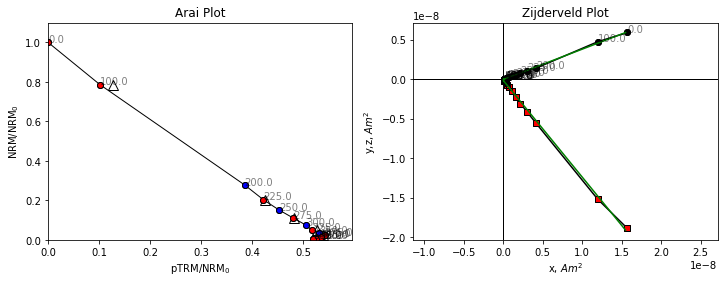
Both our Arai plot and Zijderveld plot are a straight line. Because we’re plotting magnetization lost in zero field, against magnetization gained in a known field, the ratio of our two lines is the ratio of the Ancient field to the Lab field which is a little under 2. We can check the lab field using the B_lab attribute of the specimen.
specimen.B_lab
20.0
The lab field was 20 μT. If we expect a value of 36.4 μT, then a slope of slightly under 2 is what we might expect. Let’s look at another specimen.
specimen=site['hw126a2']
fig,ax=plt.subplots(1,2,figsize=(12,4))
specimen.plot_arai(ax[0])
specimen.plot_zijd(ax[1])
ax[0].set_title('Arai Plot')
ax[1].set_title('Zijderveld Plot');
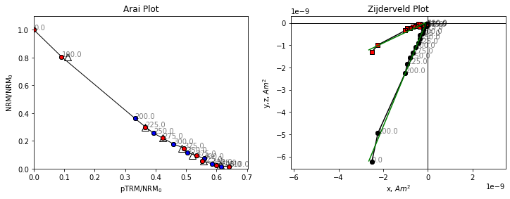
The data for this specimen do not follow a straight line. Although the line slope appears to start out at a reasonable value, it quickly becomes shallower at higher temperatures. If we were to fit a line to these data we might end up with an underestimate of the paleointensity, and there is no reason to suggest which temperature range to pick for our intensity data. Some strict selection criteria might exclude this specimen, others might include it, but could include an incorrect temperature range, which could give a biased paleointensity estimate.
The BiCEP method- accounting for bias
BiCEP works differently. It fits a circle to a scaled set of paleointensity data and uses the tangent joining the circle center and the origin. BiCEP generates many circle fits from a probability distribution. Let’s look at the circle fits that BiCEP samples from the posterior distribution, and the median tangent which we use to fit the line. BiCEP fits are performed at a site level for a reason which will become apparent later. We can use the method site.BiCEP_fit() to fit the BiCEP method (this may take several minutes depending on the speed of your processor and memory available) and plot the circle and tangent fits to the data.
#There is also a model_circle_slow which fits these circles using a slower model,
#use this if you are having problems with sampling.
site.BiCEP_fit(model=BiCEP.model_circle_fast)
#This cell may generate warnings from the internal pystan code.
#The main error to watch for is one about R_hat, which indicates the sampler hasn't converged, a "bad" run
WARNING:pystan:938 of 60000 iterations ended with a divergence (1.56 %).
WARNING:pystan:Try running with adapt_delta larger than 0.8 to remove the divergences.
We can use the specimen.plot_circ() method to draw a circle under the Arai plot data
fig,ax=plt.subplots(1,2,figsize=(12,4))
specimen.plot_circ(ax[0],tangent=True)
specimen.plot_arai(ax[0])
specimen.plot_zijd(ax[1])
ax[0].set_title('Arai Plot')
ax[1].set_title('Zijderveld Plot');
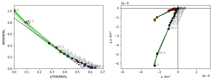
We notice that this tangent is slightly less than the initial slope, how does this help us?
BiCEP assumes that the curvature, \(\vec{k}\) (1/radius with sign depending on direction of curvature, Paterson, 2011) of the circle fit is proportional to the calculated ancient field (\(B_{anc}\)). For \(\vec{k}=0\), our “circle” has infinite radius, and so becomes a perfect line. BiCEP tries to fit a linear relationship between \(B_{anc}\) and \(\vec{k}\) for all specimens in a site. The \(B_{anc}\) value can be extrapolated (or interpolated) to \(\vec{k}\)=0 to give us our unbiased paleointensity estimate. In the case of the plotted specimen hw126a2, BiCEP predicts that this specimen should underestimate the site paleointensity slightly, due to its curvature.
We can plot the relationship between \(B_{anc}\) and \(\vec{k}\) using the method site.regplot(). We plot the expected field value as a red line.
fig,ax=plt.subplots()
site.regplot(ax)

#x limits, y limits and y label are not set by this method as it is used slightly differently in our GUI.

ax.set_xlim(-0.2,1.2)
ax.set_ylim(15,50);
ax.set_ylabel('$B_{anc}$ ($\mu$T)')
ax.axhline(36.4,color='r',zorder=0);
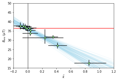
The green dots with black errorbars are our individual specimen estimates for \(\vec{k}\) and \(B_{anc}\) and their 95% confidence intervals. The blue lines are our BiCEP fits to these data. Notice that these lines cross the \(\vec{k}=0\) line close to the expected field value, yielding an accurate and precise estimate of the paleointensity, without excluding any specimens! We can get a sense of the distribution of estimates for \(B_{anc}\) using the site.histplot() method.
fig,ax=plt.subplots()
site.histplot(ax)

ax.set_xlim(30,40)
ax.axvline(36.4,color='r');
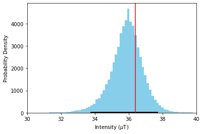
We can see that our estimate for \(B_{anc}\) is close to the median value of this distribution, and well within the 95% confidence interval denoted by the black line. Our estimate is accurate and precise, with a 95% confidence interval of ~4 μT
Data manipulation and choosing interpretations.
You might notice that some of our specimens have larger error bars on their \(\vec{k}\) estimates than others in our BiCEP fitting figure. Let’s investigate what’s going on with these specimens.
fig,ax=plt.subplots(1,2,figsize=(12,4));
hw126a7=site['hw126a7']
hw126a8=site['hw126a8']
hw126a7.plot_circ(ax[0],tangent=True)
hw126a7.plot_arai(ax[0])
ax[0].set_title('hw126a7')

hw126a8.plot_circ(ax[1],tangent=True)
hw126a8.plot_arai(ax[1])
ax[1].set_title('hw126a8');
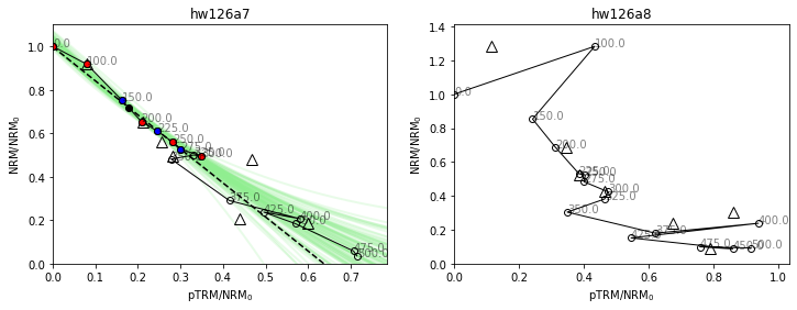
For these specimens, our analysis might be slightly different. Our specimen “hw126a7” has a pTRM check (triangle) which is very displaced from the line at the 300 °C temperature step. This is a repeat of the 300 °C in-field measurement after heating to 350 °C in zero field. It indicates a chemical alteration of the specimen between 300 °C and 350 °C. We can use this by calculating the DRAT statistic (Selkin & Tauxe, 2000), using the attribute specimen.drat, and noticing that it is high (criteria vary, but 15 is considered a high value by any metric). Although we have already demonstrated the effectiveness of BiCEP without using this statistic, we have evidence that we should only be using the temperatures up to 300 °C for this specimen. We can do this using the method specimen.change_temps(), and we save this change using the method specimen.save_changes(). Note that our attributes, such as specimen.drat are affected by the change in temperatures.
Our specimen “hw126a8” has a very early failed pTRM check, and fitting a circle seems like it would probably be inappropriate. We can elect to exclude this specimen as no part of the line is likely to give a good paleointensity estimate. This can be done by setting the attribute specimen.active=False Ultimately, due to its large uncertainty in the circle fit, it has very little effect on the estimate of \(B_{anc}\) in the first place.
The MAD statistic of Kirshvink (1980) and the DANG Statistic (Tanaka & Kobayashi, 2003, Tauxe & Staudigel, 2004) are also available using the methods specimen.mad and specimen.dang.
#Printing the DRAT parameter of the specimen to
print('hw126a7 DRAT: %2.1f'%hw126a7.drat)
print('hw126a8 DRAT: %2.1f'%hw126a8.drat)

lowerTemp=0
upperTemp=300
lowerTempK,upperTempK=lowerTemp+273,upperTemp+273

hw126a7.change_temps(lowerTempK,upperTempK)
hw126a7.save_changes()
hw126a8.active=False
hw126a7 DRAT: 4.2
hw126a8 DRAT: 38.4
We now run the BiCEP method again with these changes in place, and plot up our site results with the results for these two specimens.
site.BiCEP_fit(model=BiCEP.model_circle_fast)
WARNING:pystan:947 of 60000 iterations ended with a divergence (1.58 %).
WARNING:pystan:Try running with adapt_delta larger than 0.8 to remove the divergences.
#set up subplots
fig,ax=plt.subplots(2,2,figsize=(12,8))

#Plot our Arai plots with circle fits
hw126a7.plot_circ(ax[0,0])
hw126a7.plot_arai(ax[0,0])

hw126a8.plot_circ(ax[0,1])
hw126a8.plot_arai(ax[0,1])


#Plot our plot of the BiCEP fit.
site.regplot(ax[1,0])
ax[1,0].set_xlim(-0.2,1.2)
ax[1,0].set_ylim(15,50);
ax[1,0].set_ylabel('$B_{anc}$ ($\mu$T)')
ax[1,0].axhline(36.4,color='r',zorder=0);


#Plot our histogram
site.histplot(ax[1,1])
ax[1,1].set_xlim(30,40)
ax[1,1].axvline(36.4,color='r');
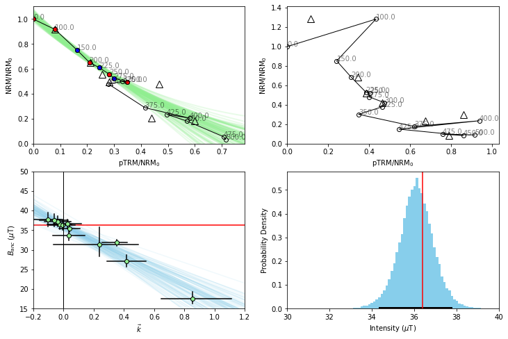
We notice from our histogram that doing this data manipulation has very slightly improved our accuracy and precision- but the overall distribution has not changed vary much. We notice from our Arai plot for specimen hw126a7 that the uncertainty in our circle fits has become much larger by excluding these temperature steps. This is because we assume the uncertainty in the circle fit for the whole Arai plot, rather than just the segment we’re looking at. In this way, we are penalized for excluding data from the Arai plot, without having to use some kind of “length of the line” criterion.
Saving data to MagIC format.
Once we have run our site- we can save our results directly into the MagIC formatted data file. This will save results of the BiCEP method for our site and all specimens in that site. We can do this using the method
site.save_magic_tables()
site.save_magic_tables()
30  records written to file  sites.txt
566  records written to file  specimens.txt
GUI
As we think that using these functions for every site will be cumbersome, we present a GUI which performs all of these steps. The GUI can save figures produced, and also produces diagnostics about the sampler, as well as important diagnostic information about the sampler. We can use the run_gui() function to initialize the GUI. Note that the %matplotlib widget magic command is required to have the BiCEP GUI display plots correctly. Above figures can be set to the normal plotting style when rerunning cells using the %matplotlib inline magic command.
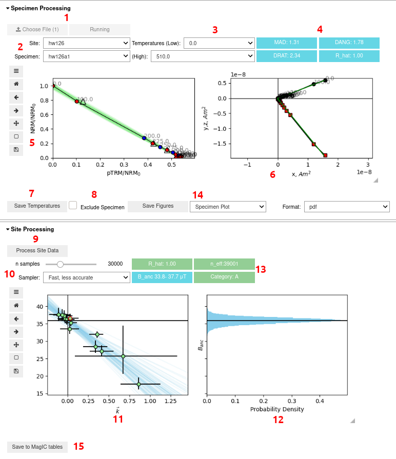
Image('readme_image/GUI_layout.png')
GUI Documentation
On launch you should have a GUI with the above layout:
File selection button. Press select, choose your file, and press select again. Then press “Run” to import the data to the GUI. You cannot then select a new file.
Site and specimen dropdowns. These dropdown menus allow you choose a particular paleointensity experiment.
Minimum and maximum temperature steps (in Celcius) to use for the paleointensity experiment. We recommend using the Zijderveld plot (7.) and pTRM checks to choose which set of temperatures to use. By default, we use all temperature steps to make a paleointensity estimate. Currently it is required to make an estimate for all specimens.
Statistics about the direction and alteration of the ChRM used for paleointensity estimation. These may help with choosing which set of temperature steps to use. See the standard paleointensity definitons (Paterson et al, 2014, https://earthref.org/PmagPy/SPD/DL/SPD_v1.1.pdf) for more information on these statistics. In addition to these statistics, we present the worst R_hat diagnostic for a specimen. If R_hat>1.1 or R_hat<0.9, it may indicate an issue with the sampler (see 13.). In this case, this box will show up as red, and the specimen may be excluded using the checkbox (8.))
Arai plot with zero field first steps plotted as red circles, in field first steps plotted as blue circles, pTRM checks plotted as triangles, and pTRM tail checks plotted as squares. Additivity checks are not currently plotted. Circle fits from the BiCEP method will be plotted as green lines under the Arai plot after the site fit (9) has been performed. All plots can be rescaled using the “move” button (3rd symbol from the bottom on left side of plot) and right clicking and dragging, or the “zoom” button (2nd symbol from the bottom) and left clicking and dragging to zoom in, or right clicking and dragging to zoom out. The “home” button (second symbol from the top) resets the plot axis, as does changing the temperatures.
Zijderveld plot of the data, with x,y plotted as black circles and x,z plotted as red squares.
Saves the temperatures used for that specimen to RAM. This must be done for each specimen individually to change temperatures before running the sampler (9.). By default, all temperature steps are used for every specimen.
Checkbox for excluding a specimen. This should only be done if there is no reasonable interpretation of the specimen (e.g. alteration at low temperature, not demagnetizing to the origin).
The “Process Site Data” button performs the BiCEP method on that site and calculates the site level paleointensity. Depending on the speed of your computer and the sampler parameters used (10), this may take a while to run, especially for sites with many specimens. Please be patient.
Parameters for the MCMC sampler for the BiCEP method. The “n samples” slider increases the number of samples used in the MCMC sampler. Smaller numbers will take less time to run but result in lower accuracy in the resulting probability distribution. The “Sampler” button changes the parameterization of the MCMC sampler slightly (mathematically, the model is the same, but the parameters being sampled from are specified slightly differently). The “Slow, more accurate” sampler is much slower than the “Fast, less accurate” sampler, but generally (though not always) results in better sampler diagnostics than the “Fast, less accurate” sampler, particularly for sites with small numbers of specimens.
Plot of the estimated paleointensity for each specimen against Arai plot curvature. The currently displayed specimen in the Arai and Zijderveld plots has a red circle around it in this plot. The blue lines are samples from the posterior distribution for the relationship between specimen level paleointensity and curvature. The y intercept is the estimated site level paleointensity.
Histogram of the site level paleointensities sampled from the posterior distribution. This corresponds to the distribution of intercepts of the blue lines in (12.).
Diagnostics for the MCMC sampler (see Cych et al, in prep. or the Stan Documentation at https://mc-stan.org/docs/2_26/reference-manual/notation-for-samples-chains-and-draws.html, https://mc-stan.org/docs/2_26/reference-manual/effective-sample-size-section.html). 0.9<R_hat<1.1 and n_eff>1000 is desired, with R_hat=1.00 and n_eff>10000 being ideal. Tweak the sampler parameters (10.) or measure more specimens if these parameters give poor results (indicated by an amber color for n_eff<1000 or a red color for bad R_hat). Also displayed here is the 95% credible interval for the site and the Category (see Cych et al once again for an explanation). The color of the category box indicates how to proceed. Green (Category A or B): Accept site, Amber (Category C or D): Measure more specimens, Red (Category D): Ignore site.
Saves figures to file. Currently the Zijderveld plot and Arai plot have to be saved together (as do both site plots).
Saves the results from the BiCEP method to the MagIC tables (site and specimen tables are altered).
%matplotlib widget
BiCEP.run_gui();
Data References and Expected Field Values
We follow with a list of DOIs for sites included in our data file as well as the expected field values at those sites. This can be useful for comparison when using BiCEP_GUI.
site_info=pd.read_csv('site_info.txt')
site_info
| Site Name | doi | Lithology | LAT | LON | Year | B_exp | n_site | |
|---|---|---|---|---|---|---|---|---|
| 0 | 1991-1992 Eruption Site | 10.1029/2005GC001141 | lava flow | 9.80000 | -104.30000 | 1991.0 | 36.2 | 53 |
| 1 | hw108 | 10.1016/j.pepi.2014.12.007 | lava flow | 19.86270 | -155.90850 | 1859.0 | 39.3 | 23 |
| 2 | hw123 | 10.1016/j.pepi.2014.12.007 | lava flow | 19.07262 | -155.71410 | 1907.0 | 37.7 | 12 |
| 3 | hw126 | 10.1016/j.pepi.2014.12.007 | lava flow | 19.69000 | -155.46000 | 1935.0 | 36.4 | 13 |
| 4 | hw128 | 10.1016/j.pepi.2014.12.007 | lava flow | 19.26000 | -155.87000 | 1950.0 | 36.2 | 26 |
| 5 | hw201 | 10.1016/j.pepi.2014.12.007 | lava flow | 19.36000 | -154.97000 | 1990.0 | 35.2 | 12 |
| 6 | hw226 | 10.1016/j.pepi.2014.12.007 | lava flow | 19.64000 | -155.51000 | 1843.0 | 39.9 | 11 |
| 7 | hw241 | 10.1016/j.pepi.2014.12.007 | lava flow | 19.52000 | -155.81000 | 1960.0 | 36.0 | 18 |
| 8 | BR06 | 10.1016/j.pepi.2007.10.002 | brick | 60.10000 | 24.90000 | 1906.0 | 49.7 | 3 |
| 9 | P | 10.1029/2010JB007844, 2011 | lava flow | 19.30000 | -102.10000 | 1943.0 | 44.6 | 36 |
| 10 | VM | 10.1029/2010JB007844, 2013 | lava flow | 40.80000 | 14.50000 | 1944.0 | 43.8 | 18 |
| 11 | BBQ | 10.1029/93jb01160 | submarine lava flow | 9.80000 | -104.30000 | 1990.0 | 36.2 | 12 |
| 12 | rs25 | 10.1016/j.epsl.2009.12.022 | synthetic | NaN | NaN | NaN | 30.0 | 5 |
| 13 | rs26 | 10.1016/j.epsl.2009.12.022 | synthetic | NaN | NaN | NaN | 60.0 | 5 |
| 14 | rs27 | 10.1016/j.epsl.2009.12.022 | synthetic | NaN | NaN | NaN | 90.0 | 10 |
| 15 | remag-rs61 | 10.1016/j.epsl.2011.08.024 | synthetic | NaN | NaN | NaN | 40.0 | 6 |
| 16 | remag-rs62 | 10.1016/j.epsl.2011.08.024 | synthetic | NaN | NaN | NaN | 60.0 | 6 |
| 17 | remag-rs63 | 10.1016/j.epsl.2011.08.024 | synthetic | NaN | NaN | NaN | 80.0 | 5 |
| 18 | remag-rs78 | 10.1016/j.epsl.2011.08.024 | synthetic | NaN | NaN | NaN | 20.0 | 4 |
| 19 | kf | 10.1111/j.1365-246X.2012.05412.x | lava flow | 65.70000 | -16.80000 | 1984.0 | 52.0 | 3 |
| 20 | Hawaii 1960 Flow | 10.1046/j.1365-246X.2003.01909.x | lava flow | 19.52000 | -155.81000 | 1960.0 | 36.0 | 22 |
| 21 | SW | 10.1016/j.pepi.2008.03.006 | lava flow | 31.60000 | -130.60000 | 1946.0 | 46.4 | 19 |
| 22 | TS | 10.1016/j.pepi.2008.03.006 | lava flow | 31.60000 | -130.60000 | 1914.0 | 47.8 | 53 |
| 23 | ET1 | 10.1016/j.epsl.2007.03.017 | basaltic lava | 37.80000 | 15.00000 | 1950.0 | 43.3 | 3 |
| 24 | ET2 | 10.1016/j.epsl.2007.03.017 | basaltic lava | 37.80000 | 15.00000 | 1979.0 | 44.1 | 2 |
| 25 | ET3 | 10.1016/j.epsl.2007.03.017 | basaltic lava | 37.80000 | 15.00000 | 1983.0 | 44.2 | 4 |
| 26 | Synthetic60 | 10.1016/S1474-7065(03)00122-0 | synthetic | NaN | NaN | NaN | 60.0 | 7 |
| 27 | LV | 10.1029/2009JB006475 | Lithic Clasts | -23.35261 | 67.74319 | 1993.0 | 24.0 | 45 |
| 28 | MSH | 10.1029/2009JB006475 | Lithic Clasts | 46.24550 | -122.18650 | 1980.0 | 55.6 | 19 |
| 29 | FreshTRM | 10.1029/2018GC007946 | remagnetized/synthetic | NaN | NaN | NaN | 70.0 | 24 |
References
List relevant references:
Cromwell, G., Tauxe, L., Staudigel, H., & Ron, H.(2015). Paleointensity estimates from historic and modern hawaiian lava flows using glassy basalt as a primary source material. Phys. Earth Planet. Int., 241, 44–56. doi:89710.1016/j.pepi.2014.12.007
Kirschvink, J. L. (1980), The least-squares line and plane and the analysis of palaeomagnetic data,Geophys. J. R. Astr. Soc.,62, 699–718, doi:10.1111/j.1365-246X.1980.tb02601.x
Nagata, T., Arai, Y., & Momose, K. (1963). Secular variation of the geomagnetic total force during the last 5000 years. J. Geophys. Res.,68(18), 5277-5281. doi:0.1029/j.2156-2202.1963.tb00005.x
Paterson, G. A. (2011), A simple test for the presence of multidomain behaviour during paleointensity experiments,J. Geophys. Res.,116, B10,104, doi:10.1029/2011JB008369.
Paterson, G. A., L. Tauxe, A. J. Biggin, R. Shaar, and L. C. Jonestrask (2014), On im-proving the selection of thellier-type paleointensity data,Geochem. Geophys. Geosyst., doi:10.1002/2013GC005135.
Selkin, P. A., and L. Tauxe (2000), Long-term variations in palaeointensity, Phil. Trans. R. Soc.London,358, 1065–1088, doi:10.1098/rsta.2000.0574.
Tanaka, H., and T. Kobayashi (2003), Paleomagnetism of the late Quaternary Ontake Volcano,Japan: directions, intensities, and excursions,Earth Planets Space,55, 189–202.
Tauxe, L., and H. Staudigel (2004), Strength of the geomagnetic field in the Cretaceous Normal Superchron: New data from submarine basaltic glass of the Troodos Ophiolite,Geochem. Geophys.Geosyst.,5, Q02H06, doi:10.1029/2003GC000635
Zijderveld, J. D. A.(1967).A. c. demagnetization of rocks: Analysis of results. In D. W. Collinson, K. M. Creer, & S. K. Runcorn (Eds.), Developments in solid earth geophysics (Vol. 3, pp. 254–286). Elsevier. doi:102110.1016/B978-1-4832-2894-5.50049-5