Exploring Research Data Repositories with geoextent
Authors
Author1 = {“name”: “Sebastian Garzón”, “affiliation”: “Opening Reproducible Research, Institute for Geoinformatics, University of Münster, Germany”, “email”: “jgarzon@uni-muenster.de”, “orcid”: “https://orcid.org/0000-0002-8335-9312”}
Author2 = {“name” : “Daniel Nüst”, “affiliation”: “Opening Reproducible Research, Institute for Geoinformatics, University of Münster, Germany”, “email”: “daniel.nuest@uni-muenster.de”, “orcid”: “https://orcid.org/0000-0002-0024-5046”}
Table of Contents
- Exploring Research Data Repositories with geoextent
- Setup
- Parameter definitions
- Data import
- Data processing and analysis
- geoextent usage
- Case study
- Analysis
- Load data
- Extraction results
- Figure 1. Repository extraction status by parameter
- Table 2. Repository extraction status by parameter
- Figure 2. Files extraction status by parameter
- Table 3. Files extraction status by parameter
- Figure 3. Geospatial extraction status by potential files
- Table 4. Geospatial extraction by files
- Figure 4. Geospatial extraction status by repositories with potential files
- Table 5. Geospatial extraction by repositories
- Figure 5. Files distribution over repositories
- Table 6. Distribution of the number of files by repositories.
- Figure 6. Percentage of potential geospatial files and success rate of extraction
- Figure 7. Success rate of extraction by file format
- Visualization of extracted geospatial extents
- References
Purpose
This notebook presents geoextent, a Python library for reliably extracting the geospatial and temporal extents of files, directories, and repository records. The geospatial and temporal metadata of research data could greatly benefit the discovery of relevant and related datasets (Gregory et al., 2018). However, it is underused in scientific data repositories except for specialised repositories. Much more scientific disciplines collect data and publish work that has some temporal or spatial relation. These datasets may not be connected through regular search indices based on keywords or full texts. The library geoextent presented in this notebook helps to understand the potential of extract information from files shared in data repositories and may be used to integrate geospatial and temporal metadata into repository infrastructures.
Technical contributions
The geoextent library is a wrapper around the most commonly used software for geospatial data loading and saving, GDAL (GDAL/OGR contributors, 2021). The main contribution is the ease of use of extracting discovery metadata from data files using GDAL, the handling of most common cases with defaults to support automation, the aggregation of extents for multiple files or directories, and the integration of retrieval functions for common scientific data repositories. This notebook relies on geoextent version 0.7.1 (Nüst, Garzón & Qamaz, 2021), and some helper functions are shared next to the notebook file. This notebook is developed for Python 3.6+ and a standard Jupyter environment (Kluyver et al., 2016). Some cells require a stable connection to the Zenodo API.
Methodology
We performed a case study of Zenodo records to explore the potential of automatically extractable geographic coverage metadata in research data repositories. Furthermore, the case study validated the features of geoextent and improved the automated handling of data types. First, a set of records based on the search term ‘geology&geo’ and below a record 500 MB size limit are downloaded, and metadata are extracted with geoextent. Results are stored in a local GeoPackage file and then analyzed. We determine the percentage of records where geospatial metadata can be automatically extracted and render the extracted geospatial and temporal metadata for visual inspection. Second, we analyze the distribution of total files and the success rate of extraction by repositories. Finally, we determine the proportion of potential files with geospatial data and its success rate of extraction.
Results
The extraction of geospatial and temporal information performed with geoextent suggests that files stored in repositories could fill gaps in the metadata of research data repositories. On the one hand, our approach to extract geographic coverage metadata generates a bounding box (bbox) for 14.4% (see Fig. 1). of the repositories explored without any manual intervention. This number is considerably higher than the current 0.77% of zenodo records with geometadata (locations) and 0.14% specifically for dataset records, though our search uses a filtered baseline for geospatial records. For the extraction of temporal extent (tbox), the successful extractions with geoextent are considerably lower with only 2.51% (see Fig. 1). This can be ascribed to time data being less explicitly modeled in common file formats compared to location data. Differences between geospatial and temporal information extractions over the total number of files (see Fig. 1) could result from file formats that reduce the ambiguity of the information only for geographical features (e.g., shp or tif). Nevertheless, these temporal extents could complement the Zenodo dates parameter, which only concerns the publication time.
As the main observation about the explored records, we found that almost 50% of files have a format known to be able to store geospatial information (‘geoformats’) (see Fig. 3). These include standardized file types for geographical information, such as GeoJSON, GeoPackage, NETCDF, and GeoTIFF, as well as other less standardized but widely used formats as CSV or png. We encountered that in terms of records, 51% have at least one file known to possibly store geospatial data. That implies that almost half of the records analyzed do not model location information in their content so that it could be extracted automatically. From the portion of records with at least one geospatial format, only 28% had a successful extraction (see Fig. 4). These observations point out the two main challenges of our approach: absence of data to explore (i.e., no geoformats in records) and low extraction success rate from available data (i.e., potential geoformats not providing the required information).
As for the files’ distribution in the repositories, we encountered that geoformats are present in repositories of all sizes and follow a similar distribution as the total number of files by records (see Fig. 5). For the repositories with successful extractions, we encountered that a single success is the most common output. However, the extraction of few repositories can rely on up to 180 successful file extractions (see Fig. 5). This number of successes is only relevant if analyzed in the context of each repository and compared with the total number of files and potential files with geospatial information. We encountered that we extracted geospatial information either in records with a low and high proportion of geoformats. A similar scenario resulted in different proportions of successful extractions from the number of geoformats (see Fig. 6). Records with no extraction (i.e., 0% success rate over potential) vary from 0% to 100% geoformat files. That suggests that there is still space for improvement for geoextent in the case of ambiguous files to increase the total percentage of successful extractions.
The proportion of success by geoformats indicates that, as expected, ambiguous formats as CSV and png are a large part of the unsuccessful extractions (see Fig. 7). As these formats do not necessarily store geographical information (e.g., can hold anything from survey data to DNA sequences) or the geographical information is not easily detectable (e.g., unexpected column names for latitude and longitude), it would be necessary to manually analyze their content to determine a perfect test dataset and possibly provide more rules for automatic extraction. In contrast, standardized formats for geographical data have a higher success rate of extraction. That confirms that these files store geospatial features in a more accessible way to other researchers than ambiguous formats. However, popular geospatial formats as GeoPackage, shapefile, or GeoTIFF have success extraction rates between 43% and 58% indicating that even standardized formats do not guarantee the availability of all required information (e.g., the coordinate reference system may be missing). Similarly, a powerful format such as netCFD (.nc) has a low extraction rate (6.6%) which shows that while it can be used for georeferenced data, it might not have sufficient metadata, or usage of non-geospatial datasets is much higher (see Fig. 7).
Finally, the bounding boxes (see Map 1 and Image 1) automatically extracted by geoextent suggest that human verification is required to identify problems with the files (e.g., incorrect or incomplete georeferencing) or with geoextent’s approach (e.g., assuming a default coordinate reference system if it is not clearly defined). Authors and data curators could easily identify common errors, e.g., flipped coordinates or absence of coordinate reference systems.

Image 1. Example of bounding boxes extracted by geoextent.(Left) Correct extraction, (Center) partially correct extraction and (Right) erroneous extraction. (Classification after human verification)
As a conclusion, we observe that the extraction of geospatial information from records in a general-purpose research data repository could provide geospatial metadata to aid data discovery. Our approach encountered potential geospatial information in a relevant percentage of repositories of different characteristics and successfully extracted geospatial information from various file types. We propose that including geoextent into the pipeline of data curation, e.g., by proposing a bounding box based on the data during record creation, could help researchers and data repositories to improve the quality of the record metadata, but also in terms of data understandability, e.g., by encouraging non-ambiguous formats.
Funding
Award1 = {“agency”: “German Research Foundation (DFG)”, “award_code”: “PE1632/17-1”, “award_URL”: ‘https://gepris.dfg.de/gepris/projekt/415851837’}
Keywords
keywords=[“geospatial”, “discovery”, “metadata”, “repositories”, “data sharing”]
Citation
Garzón, Sebastian and Nüst, Daniel, 2021. Exploring Research Data Repositories with geoextent. Accessed 2021-05-14 at https://github.com/o2r-project/geoextent/tree/master/showcase.
Suggested next steps
First, the survey of Zenodo records can be extended to include records based on more search terms - or even all records - and to include larger records. Second, the record retrieval features of geoextent can be extended to include additional research data repositories. These can be general-purpose ones, e.g., Figshare or OSF, but also specialised repositories for geospatial data, e.g., Pangaea, or GFZ Data Services. In the case of the specialised repositories, the extracted metadata should be compared with the metadata of the platform. Third, the development of geoextent will be continued, e.g., to support more data types, to support more output options for integration into other tools, or to communicate progress to users or including tools. Especially the support of more data formats and increased stability of the library could make it possible to integrate it into Open Source data repository software, such as InvenioRDM (the base software of Zenodo), and thereby turn geospatial and temporal metadata into regular record-level metadata which can be validated by authors on the creation of new records, and which can aide interdisciplinary collaboration through novel connections between datasets.
Setup
Library import
# Import geoextent
import geoextent.lib.extent as geoextent
import geoextent.lib.extent as  geoextent_help
from geoextent.__init__ import __version__ as geoextent_version
# Data manipulation
import requests
import json
from shapely import wkt
import pandas as pd
import geopandas as gpd
import numpy as np

# Logging
import logging

# Measure time and sleep function
import time

# Visualisation (graphs, maps, tables)
import matplotlib.pyplot as plt
import matplotlib as mpl
import matplotlib.ticker as mtick
import folium
from folium import plugins
from folium import  FeatureGroup, LayerControl
from folium.features import GeoJsonPopup
Local library import
# Include local library paths
import sys

# Import help functions for zenodo API
sys.path.append('help_functions')
# Import local libraries
import help_functions.request_zenodo_api as zenodo_api
Parameter definitions
# Search term for Zenodo API query
SEARCH_TERM = "geo&geology"
# Maximum size of Zenodo record to extract (MB)
MAXIMUM_RECORD_SIZE_MB = 500
# CSV output file for Zenodo API statistics
OUTPUT_API_STATISTICS = "zenodo_api_statistics.csv"
# CSV output file for search results (Zenodo record metadata)
OUTPUT_API = "zenodo_api_extraction_geo.csv"
# CSV output file for geoextent extraction results
OUTPUT_GEOEXTENT = "geoextent_extraction_geo.gpkg"
Data import
For the introductory usage examples, test data files are included in the library and available in the notebook’s repository in the tests/testdata directory, where sources of test data are documented as well. For the main analysis, data retrieval is part of the geoxtent library and therefore included in the below processing. The Zenodo record identifiers, which can be used to construct the DOI, are stored in the output dataset published next to this notebook.
Data processing and analysis
geoextent usage
Supported file types
geoextent supports a subset of the file formats supported by GDAL and uses text-scraping techniques to extract the geospatial and temporal features of common file types storing geospatial information.
This subset includes the most commonly used formats and ensures stable handling of edge cases and possible errors.
The supported file formats include vector (e.g., GeoPackage, Shapefile, GeoJSON) and raster (e.g., GeoTIFF, JPEG 2000) file types.
The user can extract the spatial extent, the so-called bounding box (parameter bbox), and/or temporal extent (parameter tbox) of a file or set of files.
Individual files
geoextent can be run on a single data file using the Python API, as shown below. The output includes the spatial and temporal extents. The spatial extent is always provided as in the WGS84 coordinate reference system (CRS), commonly known through its usage in GPS, which is sufficiently precise for the use case of dataset discovery. If the dataset is provided in a different CRS, the bounding box is reprojected using GDAL.
# File of interest
local_filepath = "../tests/testdata/shapefile/ifgi_denkpause.shp"
# Geoextent extraction
geoextent_file = geoextent.fromFile(filepath = local_filepath, bbox = True, tbox = True)

# Print output
print(local_filepath, "\n", "bbox:", geoextent_file['bbox'],"\n",geoextent_file['crs'], "EPSG \n",
     "tbox:",geoextent_file['tbox'])
../tests/testdata/shapefile/ifgi_denkpause.shp
 bbox: [7.594978277801928, 51.96852473231792, 7.5957650477781415, 51.969118924937405]
 4326 EPSG
 tbox: ['2021-01-01', '2021-01-01']
Multiple files
When provided a directory, geoextent by default returns the union of the spatial and temporal extent of all supported files.
# Directory of interest
local_directory_path = "../tests/testdata/folders/folder_two_files"
# Geoextent extraction
geoextent_directory = geoextent.fromDirectory(path = local_directory_path, bbox = True, tbox = True, details = True)

# Print output
print(local_directory_path, "\n", "bbox:", geoextent_directory['bbox'],"\n", geoextent_directory['crs'], "EPSG \n",
     "tbox:",geoextent_directory['tbox'])
../tests/testdata/folders/folder_two_files
 bbox: [2.052333387639205, 41.31703852240476, 7.647256851196289, 51.974624029877454]
 4326 EPSG
 tbox: ['2018-11-14', '2019-09-11']
The previous result is the combination of two files: muenster_ring_zeit.geojson and
districtes.geojson, so geoextent also stores (If parameter details = True ) the details from the files used to compute the final bbox and tbox. For example:
geoextent_directory['details']['muenster_ring_zeit.geojson']
{'format': 'geojson',
 'geoextent_handler': 'handleVector',
 'bbox': [7.6016807556152335,
  51.94881477206191,
  7.647256851196289,
  51.974624029877454],
 'crs': '4326',
 'tbox': ['2018-11-14', '2018-11-14']}
Data repositories
Geoextent aims to extract the bounding box (bbox) and temporal box (tbox) from data repositories. The first data repository implemented is Zenodo, and the extraction is based on either a Zenodo Record URL (e.g., https://zenodo.org/record/820562) or the URL of a DOI (e.g., https://doi.org/10.5281/zenodo.820562).
# Zenodo Record of interest
url_zenodo =  "https://zenodo.org/record/820562"
url_doi = "https://doi.org/10.5281/zenodo.820562"

# Geoextent extraction
geoextent_url_doi = geoextent.from_repository(url_doi, bbox = True)
geoextent_zenodo_record = geoextent.from_repository(url_zenodo, bbox = True)

# Print output
print(url_doi,"\n", "bbox:", geoextent_zenodo_record['bbox'],"\n")
print(url_zenodo, "\n", "bbox:", geoextent_zenodo_record['bbox'])
https://doi.org/10.5281/zenodo.820562
 bbox: [96.21146318274846, 25.558346194400002, 96.35495081696702, 25.632931128800003]

https://zenodo.org/record/820562
 bbox: [96.21146318274846, 25.558346194400002, 96.35495081696702, 25.632931128800003]
Command-line interface
Geoextent’s API functionalities are also accessible through a command-line interface (CLI) for files, folders, and data repositories. In this scenario, configuration options for the extraction are provided by flags. For example, -b indicates a bounding box (bbox) extraction, and -t a time box (tbox) extraction. Additional options are available, e.g., --details to print the individual results by file for folders and data repositories or --output to store the output in a GeoPackage file instead of printing to console.
%%bash
geoextent -b -t ../tests/testdata/shapefile/ifgi_denkpause.shp
{'format': 'shp', 'geoextent_handler': 'handleVector', 'bbox': [7.594978277801928, 51.96852473231792, 7.5957650477781415, 51.969118924937405], 'crs': '4326', 'tbox': ['2021-01-01', '2021-01-01']}
/home/garzon/.local/lib/python3.6/site-packages/pandas/compat/_optional.py:124: UserWarning: Pandas requires version '1.2.1' or newer of 'bottleneck' (version '1.2.0' currently installed).
  warnings.warn(msg, UserWarning)
Case study
Zenodo is a data repository that stores different types of publication materials in form of records. The Zenodo API supports the discovery of records by dozens of different parameters stored in the metadata. These parameters include, e.g., title, doi, keywords, and locations. Even though geospatial metadata is available for queries via the locations parameter, this option seems to be limited to only a small number of records. Therefore, we study the number of records with geospatial metadata available in Zenodo and assess if by using geoextent we could provide the missing geospatial metadata for a significant number of other Zenodo records.
Zenodo geometadata
The first step for this analysis is determining the current state of geometadata in the Zenodo records. Only Open Access repositories are taken into account. For this purpose, we are going to use the Zenodo spatial search function using the bounds query parameter, which accepts an area of interest (bounding box) as two coordinate pairs to extract the records within this zone. Zenodo’s geospatial information of a record is stored in the locations property in the metadata. Each record could have multiple locations, but a location is limited to a single point with the properties lat, lon, and place.
In the following cell, we extract the proportion of Open Access Zenodo records which have a locations property value. It is important to note that Zenodo records include 9 different categories of publication types: poster, presentation, dataset, image, video, software, lesson, physicalobject, and other, all of which are queried.
ONLY RUN THE FOLLOWING CELL IF YOU WANT THE CURRENT INFORMATION FROM ZENODO API
New records are being added every day to Zenodo. We have prepared a data frame with the results from the API at the time of our analysis.
Change the following cell type from Raw to Code before running it.
df_api = pd.read_csv(OUTPUT_API_STATISTICS,index_col=0)
df_api
| Number open access records | Number open access records with geometadata | % records with metadata | % proportion over total geometadata | |
|---|---|---|---|---|
| Type of record | ||||
| publication | 997743 | 13970 | 1.400160 | 99.849904 |
| poster | 8397 | 0 | 0.000000 | 0.000000 |
| presentation | 21225 | 0 | 0.000000 | 0.000000 |
| dataset | 75542 | 19 | 0.025152 | 0.135802 |
| image | 601753 | 0 | 0.000000 | 0.000000 |
| video | 3286 | 0 | 0.000000 | 0.000000 |
| software | 53737 | 1 | 0.001861 | 0.007147 |
| lesson | 2555 | 0 | 0.000000 | 0.000000 |
| physicalobject | 28 | 0 | 0.000000 | 0.000000 |
| other | 6168 | 1 | 0.016213 | 0.007147 |
| record | 1770435 | 13991 | 0.790258 | 100.000000 |
Table 1. Zenodo records statistics by record type
Based on the information extracted from Zenodo’s API on May 14, 2021 (08:25:00 UTM), there are 1,770,284 open records. From these records, 13,966 have geospatial metadata. That means that ~0.79% of open Zenodo records are findable through geospatial search. Among the records with geospatial metadata, ~99.8% are publications(13945, records), and ~0.14% are of dataset type (19 records). Even for these two categories with most of the records, less than 1.4% of open publications and less than 0.03% open dataset include geospatial metadata.
To evaluate if we can use geoextent to increase the proportion of records with spatial metadata, we use the result of a Zenodo API term search to create a list of records to analyze. In this particular search, we use the term geo&geology and limit it to only dataset records smaller than 500 MB. From these records’ metadata, we store basic fields, e.g., title, DOI, in the CSV file zenodo_api_extraction_geo.csv.
ONLY RUN THE FOLLOWING CELL IF YOU WANT TO REPRODUCE THE GEOEXTENT EXTRACTION
New records are being added every day to Zenodo. Some of them could match our search query after the publication of this notebook. That means that our geoextent extraction (See. Collect data) could change.
Change the following cell type from Raw to Code before running it.
Collect data
ONLY RUN THE FOLLOWING CELL IF YOU WANT TO REPRODUCE THE GEOEXTENT EXTRACTION
Change the following cell type from Raw to Code before running it. This process could take more than 3 hours.
Analysis
Load data
After the geographical and temporal extent extraction of the Zenodo repositories, we have information for repositories and files. We load the results of the geoextent extraction and split it into two GeoDataFrames, one for each type of data: gdf_repository for repositories and gdf_files for files. We also load the results of the zenodo API metadata extraction into a data frame: df_geo_zenodo_api.
# Loads results from api and geoextent extraction
df_geo_zenodo_api = pd.read_csv(OUTPUT_API, index_col=0)
df_geo_zenodo_api.index = df_geo_zenodo_api.index.astype(str)
gdf_geo = gpd.read_file(OUTPUT_GEOEXTENT)
gdf_geo = gdf_geo.rename(columns={'geometry': 'bbox'}).set_geometry('bbox')

#df_geo = pd.read_csv(OUTPUT_GEOEXTENT, index_col=0)

# Creates two different geodataframes, one for files and other for zenodo records (repositories)

geoextent_ext = gdf_geo['handler'].str.find("geoextent:") == 0
gdf_repository = gpd.GeoDataFrame(gdf_geo[geoextent_ext],geometry ="bbox",crs = 4326)
gdf_repository.drop(['filename'], axis = 1,inplace = True)
gdf_files = gpd.GeoDataFrame(gdf_geo[~geoextent_ext],geometry ="bbox",crs = 4326)
Extraction results
The extraction for each Zenodo record has three possible results:
a successful extraction
no information extracted
a failure (“error”) during the extraction.
As results can differ for the respective extraction of geospatial and temporal metadata, these properties are analyzed individually.
Figure 1. Repository extraction status by parameter
# Extract statistics for geospatial extraction

num_records = len(gdf_repository)
per_records_geoextent = sum(gdf_repository.bbox.is_valid)/num_records*100
per_records_no_geoextent = (sum(gdf_repository.format == "repository")/num_records*100) - per_records_geoextent
per_records_failure = sum(gdf_repository.format == "repository_error")/num_records*100

# Extract statistics for temporal extraction
per_records_temp = (num_records-sum(gdf_repository.tbox.isnull()))/num_records*100
per_records_no_temp = (sum(gdf_repository.tbox.isnull())-sum(gdf_repository.format == "repository_error"))/num_records*100

# Store results
rec_successful = [per_records_geoextent,per_records_temp]
rec_no_extraction = [per_records_no_geoextent,per_records_no_temp]
rec_failure =  [per_records_failure,per_records_failure]

## Plot
fig, ax = plt.subplots(figsize=(15,3))

# Plot configuration
ext_type = ["Geospatial \n extent","Temporal \n extent"]
plt.barh(ext_type, rec_successful,color='g',alpha=0.5,label ='Successful')
plt.barh(ext_type, rec_no_extraction,color='grey',alpha=0.5,label ='No extraction',left = rec_successful)
plt.barh(ext_type, rec_failure,color='red',alpha=0.5,label ='Geoextent failure',left = [sum(x) for x in zip(*[rec_successful,rec_no_extraction])])
plt.xlabel('(%) Percentage of repositories')
fig_num = 1
plt.annotate('n='+str(num_records)+' repositories', (45,0.5))
plt.annotate('Figure '+ str(fig_num)+'. Extraction results of temporal and geospatial metadata for Zenodo records',
             (0,0), (200, -40), xycoords='axes fraction', weight='bold', textcoords='offset points', va='center')
plt.annotate('https://o2r.info/geoextent/', (0,0), (710,-35), xycoords='axes fraction', textcoords='offset points', va='top')
fig_num +=1
plt.legend(loc=1)
plt.show()

# dataframe with results
df_repo_extractions = pd.DataFrame.from_dict({"% Successful extractions":rec_successful,
      "% No extraction":rec_no_extraction,
      "% Geoxtent failure": rec_failure},orient='index',columns=['Geospatial extraction', 'Temporal extraction']).transpose()

df_repo_extractions['Number success']= df_repo_extractions['% Successful extractions']/100*num_records
df_repo_extractions['Number No extractions']= df_repo_extractions['% No extraction']/100*num_records
df_repo_extractions['Number Geoextent Failure']= df_repo_extractions['% Geoxtent failure']/100*num_records
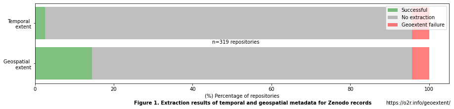
Table 2. Repository extraction status by parameter
df_repo_extractions
| % Successful extractions | % No extraction | % Geoxtent failure | Number success | Number No extractions | Number Geoextent Failure | |
|---|---|---|---|---|---|---|
| Geospatial extraction | 14.420063 | 81.191223 | 4.388715 | 46.0 | 259.0 | 14.0 |
| Temporal extraction | 2.507837 | 93.103448 | 4.388715 | 8.0 | 297.0 | 14.0 |
From a total of 319 Zenodo records analyzed, we extracted the geospatial extent from 14.42% and the temporal extent from 2.51%. geoextent did not retrieve the geospatial and temporal extent in 81.19% respectively 93.10% of the cases. That means that geoextent explored all files in those records, but did not encounter supported files to retrieve information. Finally, the extraction with geoextent failed due to unknown reasons in 4.39% of the records.
A similar analysis is possible for the individual files. In this case, only two outputs are possible:
extraction is successful
there is no extraction at all
In the following code, we first remove folders and ZIP archives from the used data subset, as the data files include both the files and the combined result for folders and ZIP archives.
Figure 2. Files extraction status by parameter
# Extract only files (no folders or zipfile)
uni_files_gdf = gdf_files[~gdf_files.format.isin(["folder","zip"])].copy().reset_index(drop=True)
uni_files_gdf.format = uni_files_gdf.format.str.lower()

# Extract statistics for geospatial extraction
num_files = len(uni_files_gdf)

# Percentage files with valid bbox (i.e., valid geometry) from total number of files
per_files_geoextent = sum(uni_files_gdf.bbox.is_valid)/num_files*100
# Percentage files without valid bbox (i.e., no geometry) from total number of files
per_files_no_geoextent = 100-per_files_geoextent

# Extract statistics for temporal extraction
per_files_temp = (num_files-sum(uni_files_gdf.tbox.isnull()))/num_files*100
per_files_no_temp = 100-per_files_temp

# Record results
files_successful = [per_files_geoextent,per_files_temp]
files_no_extraction = [per_files_no_geoextent,per_files_no_temp]

# Plot
status = ["Successful extraction","No extraction"]
fig, ax = plt.subplots(figsize=(15,3))
plt.barh(ext_type, files_successful,color='g',alpha=0.5,label ='Successful')
plt.barh(ext_type, files_no_extraction,color='grey',alpha=0.5,label ='No extraction',left = files_successful)
plt.xlabel('(%) Percentage of files')
plt.xlim(0,100)
plt.legend(status,loc=1)
plt.annotate('n='+str(num_files)+' files', (50,0.5))
plt.annotate('Figure '+ str(fig_num)+'. Extraction results of temporal and geospatial metadata for individual files from Zenodo records',
             (0,0), (120, -40), xycoords='axes fraction', weight='bold', textcoords='offset points', va='top')
plt.annotate('https://o2r.info/geoextent/', (0,0), (710,-60), xycoords='axes fraction', textcoords='offset points', va='top')
fig_num+=1
plt.show()

# dataframe with results
df_files_extractions = pd.DataFrame.from_dict({"% Successful extractions":files_successful,
      " % No extraction":files_no_extraction},orient='index',columns=['Geospatial extraction', 'Temporal extraction']).transpose()
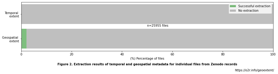
Table 3. Files extraction status by parameter
df_files_extractions
| % Successful extractions | % No extraction | |
|---|---|---|
| Geospatial extraction | 2.134463 | 97.865537 |
| Temporal extraction | 0.080909 | 99.919091 |
From 25,955 files analyzed, 0.08% had a successful temporal extraction and 2.13% a geospatial extraction. Files for which neither temporal nor geospatial metadata could be extracted are diverse. For instance, Zenodo records include non-data files (e.g., documentation, code) or data that has no geospatial component (e.g., laboratory measurements). Even for file formats designed to store geospatial data, there is a risk of ambiguity or lack of information regarding the coordinate reference systems, or geospatial data file formats may be unsupported. Therefore, we took investigated files in known geospatial data formats. This group gives us a better idea of the proportion of geospatial metadata that we could extract automatically.
Figure 3. Geospatial extraction status by potential files
# List of potential file formats with geospatial information
potential_geo_formats = ['nc', 'shp', 'shx', 'dbf', 'kml', 'gpkg', 'xls', 'gdbtable','geojson', 'gmt','gml',
                         'pdf', 'png', 'tif', 'jpg', 'nc', 'jpeg','img', 'bmp','asc', 'ovr','unw', 'h5', 'kml', 'tiff','csv']

# Extract total number of files by zenodo record
total_files = uni_files_gdf.zenodo_record_id.value_counts()

# Extract total number of potential file with geoextent by zenodo record
files_potential_geo_formats = uni_files_gdf['format'].isin(potential_geo_formats).groupby(uni_files_gdf['zenodo_record_id']).sum()

# Extract total number of files with potential geospatial information
total_files_potential = sum(files_potential_geo_formats)

# Extract percentage of files with successful geoextent extraction from the potential
per_total_geoextent_potential = sum(uni_files_gdf.bbox.is_valid) / total_files_potential * 100

## Plot
fig, ax = plt.subplots(figsize=(15,3))
# Plot configuration
plt.barh("Geoextent \n extraction",per_total_geoextent_potential,color='g',alpha=0.5,label ='Successful extraction')
plt.barh("Geoextent \n extraction",100-per_total_geoextent_potential,color='grey',alpha=0.5,label ='No extraction',left = per_total_geoextent_potential)
plt.xticks(np.arange(0,101, 5.0))
plt.xlabel('(%) Percentage of files')
plt.annotate('n='+str(total_files_potential)+" files", (45,0))
plt.annotate('Figure '+str(fig_num)+'. Geoextent extraction for known geospatial data file formats', (0,0),
             (200, -40), xycoords='axes fraction', weight='bold', textcoords='offset points', va='top')
plt.annotate('https://o2r.info/geoextent/', (0,0), (710,-40), xycoords='axes fraction', textcoords='offset points', va='top')
fig_num +=1
plt.legend()
plt.show()

# dataframe with results
df_files_extractions_from_potential = pd.DataFrame.from_dict({"Total number of files":int(num_files),
                                                              "Number of files with potential":int(total_files_potential),
                                                              "% Files with potential":100*total_files_potential/num_files,
                                                              "% Successful extractions over potential":per_total_geoextent_potential,
                                                              "% No extractions over potential":100-per_total_geoextent_potential},
                                                             orient='index',columns=['Geospatial extraction'])
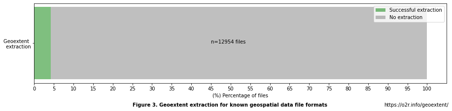
Table 4. Geospatial extraction by files
df_files_extractions_from_potential
| Geospatial extraction | |
|---|---|
| Total number of files | 25955.000000 |
| Number of files with potential | 12954.000000 |
| % Files with potential | 49.909459 |
| % Successful extractions over potential | 4.276671 |
| % No extractions over potential | 95.723329 |
From 25,955 files, there are 12,954 (49.91%) files with known formats that could potentially store geospatial information. From these files, only 4.28% had a successful geoextent extraction, i.e., a bounding box could be derived, and 95.72% resulted in no extraction. The distribution of these files among the records is relevant to explore the percentages of Zenodo records that could have a successful geoextent extraction, i.e., at least one file with successful extraction.
Figure 4. Geospatial extraction status by repositories with potential files
# Extract total number of files with successful geoextent extraction by zenodo record
geo_files = uni_files_gdf['bbox'].is_valid.groupby(uni_files_gdf['zenodo_record_id']).sum()

#Extract number of records by category
num_records_with_files = len(files_potential_geo_formats)

num_repo_potential_geo = sum(files_potential_geo_formats>0)
per_potential_geoextent = sum(geo_files>0)/num_repo_potential_geo*100
per_potential_no_geoextent = 100-per_potential_geoextent

## Plot
fig, ax = plt.subplots(figsize=(15,3))
# Plot configuration
plt.barh("Records with potential \n geospatial information",per_potential_geoextent,color= 'green',alpha=0.5,label ='Successful extraction')
plt.barh("Records with potential \n geospatial information",per_potential_no_geoextent,alpha=0.5, color = 'gray',label ='No extraction',left=per_potential_geoextent)
plt.annotate('Figure '+str(fig_num)+'. Geoextent extraction for different groups of \n Zenodo records with at least one potential file with geospatial information', (0,0),
             (160, -40), xycoords='axes fraction', weight='bold', textcoords='offset points', va='top')
plt.annotate('https://o2r.info/geoextent/', (0,0), (710,-40), xycoords='axes fraction', textcoords='offset points', va='top')
plt.annotate('n='+str(num_repo_potential_geo), (50,0))
plt.xlabel('(%) Percentage of zenodo records')
plt.legend()
fig_num +=1
ax.xaxis.set_major_formatter(mtick.PercentFormatter())
plt.show()

# dataframe with results
df_repos_extractions_from_potential = pd.DataFrame.from_dict({"Total repositories":int(num_records),
                                                              "Repositories explored":int(num_records_with_files),
                                                              "Number of repositories with potential":int(num_repo_potential_geo),
                                                              "% Repositories with potential":100*num_repo_potential_geo/num_records,
                                                              "% Successful extractions over potential":per_potential_geoextent,
                                                              "% No extractions over potential":per_potential_no_geoextent},
                                                             orient='index',columns=['Geospatial extraction'])
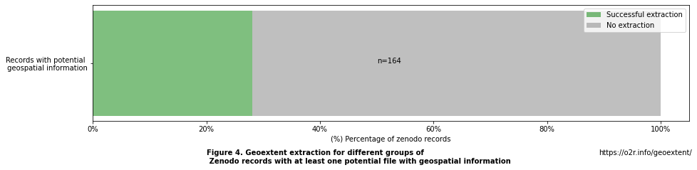
Table 5. Geospatial extraction by repositories
df_repos_extractions_from_potential
| Geospatial extraction | |
|---|---|
| Total repositories | 319.000000 |
| Repositories explored | 301.000000 |
| Number of repositories with potential | 164.000000 |
| % Repositories with potential | 51.410658 |
| % Successful extractions over potential | 28.048780 |
| % No extractions over potential | 71.951220 |
From the 301 Zenodo records analyzed, 164 have at least one file with a supported file format. Consequently, in the best scenario, the percentage of successful geospatial extraction on the level of records would be 51.41%. However, from the 164 repositories with potential files, only 28.05% of records could be attributed to a geospatial extent (i.e., 14.42% over total records).
To understand the problem better, we next explore the distribution of files per repository. Specifically, exploring the total number of files, the number of potential successful extractions (i.e., supported file formats), and the actual number of successful extractions.
Figure 5. Files distribution over repositories
# Define plot
fig, ax = plt.subplots(figsize=(15,5))
# Extract bins in logaritmic scale
f = uni_files_gdf.zenodo_record_id.value_counts()
hist, bins = np.histogram(f, bins=12)
logbins = np.logspace(np.log10(bins[0]),np.log10(bins[-1]),len(bins))
# Includes 0 into the 'logaritmic' scale
bin_dist = np.append([-0.1],logbins)

# Plot distribution of 3 categories in common sudo-logaritmic (zero-included) scale
total_files.hist(ax = ax, bins=bin_dist,alpha=0.3,color = 'blue',edgecolor="blue", grid=False, label = "Total files")
files_potential_geo_formats.hist(ax=ax,alpha=0.5, color = 'orange',edgecolor="black",hatch = '*',grid=False,bins=bin_dist, label = "Potential files with geoextent")
geo_files.hist(ax= ax,histtype='barstacked',color= 'green',edgecolor="black",hatch = 'x',alpha=0.7,grid=False,bins=bin_dist, label = "Files with geoextent")

# Plot configuration
plt.ylabel('Number of repositories (Count)')
plt.xlabel('Number of files  (Equally-space logaritmic)')
plt.xscale('log')
plt.yscale('log')
plt.gca().yaxis.set_major_formatter(mpl.ticker.ScalarFormatter())
plt.gca().xaxis.set_major_formatter(mpl.ticker.ScalarFormatter())
plt.yticks([1,2,5,10,20,50,100,200])
plt.xticks([1,2,5,10,20,50,100,200,500,1000,2000,5000,1000])
plt.annotate('Figure '+str(fig_num)+'. Potential and successful files for geospatial metadata extration\n across Zenodo repositories with different number of files', (0,0),
             (200, -40), xycoords='axes fraction', weight='bold', textcoords='offset points', va='top')
plt.annotate('https://o2r.info/geoextent/', (0,0), (710,-50), xycoords='axes fraction', textcoords='offset points', va='top')
fig_num +=1
plt.legend(loc=1, prop={'size': 12})
plt.show()
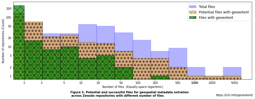
Table 6. Distribution of the number of files by repositories.
pd.DataFrame(list(zip(total_files.describe()[1:],files_potential_geo_formats.describe()[1:],geo_files.describe()[1:])),
            columns =['Files in repository', 'Potential files with geoextent','Files with geoextent'],
            index=['Mean','Standard deviation','Min','25%','50%','75%','Max'])
| Files in repository | Potential files with geoextent | Files with geoextent | |
|---|---|---|---|
| Mean | 86.229236 | 43.036545 | 1.840532 |
| Standard deviation | 457.793327 | 400.699765 | 11.620147 |
| Min | 1.000000 | 0.000000 | 0.000000 |
| 25% | 3.000000 | 0.000000 | 0.000000 |
| 50% | 12.000000 | 1.000000 | 0.000000 |
| 75% | 31.000000 | 4.000000 | 0.000000 |
| Max | 6515.000000 | 6515.000000 | 180.000000 |
We can observe that for the distribution of the total number of files in Zenodo records, there are on average 86.23 files with a standard deviation of 457.79. As suggested by the high standard deviation, there are a few records with a very high number of files. A better way to describe the number of files by repository is by quantiles. For example, 50% of the records have less than 12.0 files.
In the figure, we can see that supported files are found in repositories with varying numbers of files. There are 43.04 files on average with potential geospatial information with a standard deviation of 400.7. As before, a better indicator of the distribution results from the quantiles. For this case, 50% of the repositories have less than 1.0 file with a supported file format. 137 records of the 319 analyzed have 0 supported files.
Regarding successful extractions, there are 1.84 files on average with geoextent per repository analyzed with a standard deviation of 11.62. In total 255 records did not have a successful geoextent extraction. For repositories with successful extraction, we can see that the final geospatial extraction relies in some cases on only 1 file extraction result, yet in one case on 180 file extractions.
To understand the types of Zenodo records that result in a successful geoextent extraction, we computed the proportion of files with potential geospatial information over the total number of files and the percentage of files with successful extraction over the potential.
Figure 6. Percentage of potential geospatial files and success rate of extraction
# Extract number of total files by records with successful extraction by zenodo record
files_in_record = uni_files_gdf.zenodo_record_id.value_counts()
# Extract number of files with successful extraction with potential geospatial information by zenodo record
potential_files_with_geo_in_record = uni_files_gdf['format'].isin(potential_geo_formats).groupby(uni_files_gdf['zenodo_record_id']).sum()
# Extract number of files with successful geoextent extraction by zenodo record
files_with_geo_in_record = uni_files_gdf['bbox'].is_valid.groupby(uni_files_gdf['zenodo_record_id']).sum()

# Store information
result = pd.DataFrame({'files_in_record': files_in_record,
                       'files_with_potential_geoextent': potential_files_with_geo_in_record,
                       'files_with_extracted_geoextent': files_with_geo_in_record,
                      })

result['per_success_from_total'] = result.files_with_extracted_geoextent/result.files_in_record*100
result['per_success_from_potential'] = result.files_with_extracted_geoextent/result.files_with_potential_geoextent*100
result['potential_per_success'] = result['files_with_potential_geoextent']/result['files_in_record']*100

# This line includes repositories with 0 potential files. Replace NaN to 0
# All repos without potential files go to (0,0)
result.per_success_from_potential.fillna(0, inplace=True)

## Plot

fig, ax = plt.subplots(figsize=(15,8))

scatter = plt.scatter(result['potential_per_success'],result['per_success_from_potential'],
                     c=result['per_success_from_total'], s=result['files_in_record'], cmap="copper",alpha= 0.7)

range_per_success_total = list(np.arange(0.0,120,20))

# produce a legend with the unique colors from the scatter
plt.colorbar(label="Percentage of successful extraction \n over total files in repository")

range_num_files = list(result['files_in_record'].quantile([0.1,0.3,0.6,0.8,0.9,0.99]).round(0))

# produce a legend with a cross section of sizes from the scatter
kw = dict(prop="sizes", num=range_num_files, fmt="{x:,}", func=lambda s: s,alpha=0.5)
legend2 = ax.legend(*scatter.legend_elements(**kw),title="# of total files \n in record" ,bbox_to_anchor=(0.15,0.9))
plt.ylim(-1,103)
plt.xlabel('Percentage of files in repository with potential geospatial information')
plt.ylabel('Percentage of files with successful geospatial \n information extraction over potential files')
plt.annotate('Figure '+str(fig_num)+'. Potential geospatial files vs. success rate over potential', (0,0),
             (140, -40), xycoords='axes fraction', weight='bold', textcoords='offset points', va='top')
plt.annotate('https://o2r.info/geoextent/', (0,0), (600,-40), xycoords='axes fraction', textcoords='offset points', va='top')
plt.annotate("1'",xy=(42, 20), xytext=(45, 25),arrowprops=dict(arrowstyle="->"))
plt.annotate("2'", xy=(99, 99), xytext=(92, 95),arrowprops=dict(arrowstyle="->"))

fig_num +=1
plt.show()
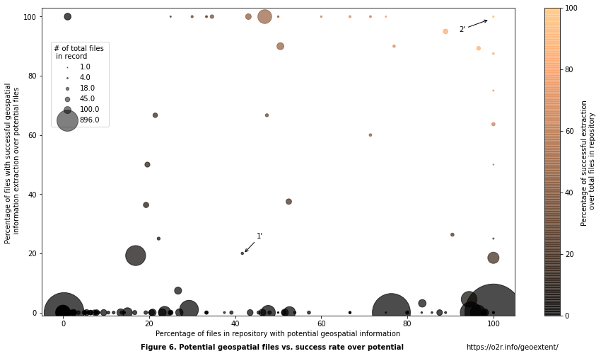
Each circle in the above figure represents a Zenodo record and its extraction results. For example, the repository Is drought tolerance a domestication trait in tepary bean?: Allelic diversity at abiotic stress responsive genes in cultivated Phaseolus acutifolius A. Gray and its wild relatives (see 1’ in the figure) has a total number of
12 files. From those files, 5 (41.67%) corresponds to a file format known to possibly store geospatial information (.CSV) and the remaining files are text files with DNA data (FAS). From these supported files, only 1 has a successful extraction resulting in a 20% of success over the potential. Another example repository, The Literary Geographies of Christine de Pizan (geo-data) (see 2’ in the figure) only has 1 file. This file is from a supported format (CSV) and the extraction was successful resulting in both potential and successful extraction of 100%. The differences between these two cases with only one successful geoextent extraction illustrate the complexity in understanding the reliability of the extraction.
In general, we observe that records with 0% successful extractions (vertical axis) over their potential (horizontal axis) have different percentages of potential geospatial information over the total number of files. That means that most of these records have a relevant (proportional to their size) number of files with formats known to contain geospatial information, but geoextent did not extract any information. As mentioned before, this could be due to ambiguous file formats (such as CSV files) that do not necessarily store geospatial information or that do so in an unsupported way. We observe that repositories with successful extraction are usually small repositories in which the potential geospatial files represent more than 20% of the total files. There are few cases in which records with successful geospatial extractions have a 100% success rate of extraction over its potential. That means that the extracted bounding box could be missing some information.
To understand which formats are problematic to extract geospatial information, we compute the percentages of extraction success.
Figure 7. Success rate of extraction by file format
uni_files_gdf['format'].value_counts()
files_valid = uni_files_gdf[uni_files_gdf.geometry.is_valid].copy().reset_index(drop=True)

d1 = pd.DataFrame({"Total":uni_files_gdf['format'].value_counts(),
                  "geoextent_success":files_valid['format'].value_counts()})
d1.dropna(inplace=True)
d1['perc_success'] = (d1['geoextent_success']/d1['Total'])*100

# To avoid repetition for shapefiles we remote dbf and shx
d1.drop('dbf',inplace=True)
d1.drop('shx',inplace=True)

labels = d1.index.values
success = d1['perc_success']
failure = 100 - d1['perc_success']

color_success = ["#009900","#255e25"]
color_failure = ["#FF3333","#930707"]
fig, ax = plt.subplots(figsize=(15,4))
width = 0.35
plt.bar(labels, success, width, label='Successful',color= color_success[0])
plt.bar(labels, failure, width, bottom=success, color = color_failure[0],label='No extraction')
plt.ylabel('Percentage')
plt.xlabel('File format')
plt.ylabel('Percentage')

count = 0
for bar in ax.patches:
    displace =-1
    color = color_failure[1]
    pos = 90
    if bar.get_y() == 0:
        n = d1['Total'][count]
        count+=1
        displace = 3
        color= color_success[1]
        pos = 0
        plt.annotate("n= "+str(n),
                   (bar.get_x() + (bar.get_width()/2),
                   50), ha='center', va='center',
                   size=10, xytext=(0, 0),color='black',
                   textcoords='offset points')
    plt.annotate(format(bar.get_height()/100, ".1%"),
                   (bar.get_x() + (bar.get_width()*1.5),
                   pos), ha='center', va='center',
                   size=10, xytext=(0, 8),color=color,
                   textcoords='offset points')

plt.legend(loc='center right', bbox_to_anchor=(1.1, 0.5))
plt.annotate('Figure '+str(fig_num)+'. Geoextent extraction success by supported file type', (0,0), (240, -40), xycoords='axes fraction', weight='bold', textcoords='offset points', va='top')
plt.annotate('https://o2r.info/geoextent/', (0,0), (710,-40), xycoords='axes fraction', textcoords='offset points', va='top')
fig_num +=1
plt.show()
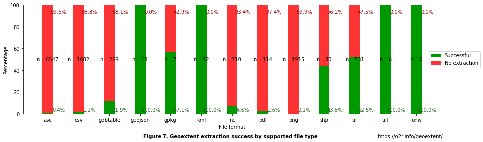
First, we can observe that file formats whose main purpose is to store geospatial information have a higher success rate of extraction. For example, GeoJSON, TIFF, KML, and UNW have a 100% success rate, but the number of files is relatively small.
Surprisingly though, other popular formats have a lower success rate (with bigger samples). For example,
GeoPackage (.gpkg), an open format for geospatial information, has a lower success rate of 57.1%. That could result from the small sample size (n=7) and errors in the formatting of files as those present in other geospatial file formats (e.g., 56.25% failure in .shp). Similarly, .shp and.tif success rates vary between 43.75 and 52.54%.
Second, the results suggest that ambiguous formats (i.e., those that do not necessarily have geospatial information) unsurprisingly have a high percentage of no extractions. For CSV files, geoextent could not extract geospatial information in 98.8% of files. To determine what percentage corresponds to information without geospatial data (e.g., laboratory results) and those with geospatial information but unsuccessful extraction, we would need to evaluate each file by hand. However, what is relevant for us is that at least 1.2% of CSV files have extractable geospatial information. Files with a .png format also have a similar low success rate of 0.10%. That means that we can not discard ambiguous file formats as potential sources of geometada.
Third, the low success rate for NetCDF.nc (6.6%) files, an array-oriented scientific data format, could suggest that information is store in multiple formats without implementing its full capabilities to preserve geospatial information. Even though the success rate of this and other specialised file formats are higher than ambiguous formats, a better performance would be desirable to store and reduce problems while reproducing the findings of the studies.
Visualization of extracted geospatial extents
For a final evaluation of the geoextent extraction, we generate a map of bounding boxes by record (repository).
Map 1. Extracted bounding boxes visualization
# Extract only repositories and files with geometry

rep_valid = gdf_repository[gdf_repository.geometry.is_valid].copy().reset_index(drop=True)
rep_valid.tbox = rep_valid.tbox.fillna("")
rep_valid.zenodo_record_id = rep_valid.zenodo_record_id.astype(str)

files_valid = uni_files_gdf[uni_files_gdf.geometry.is_valid].copy().reset_index(drop=True)
files_valid.zenodo_record_id = files_valid.zenodo_record_id.astype(str)

rep_valid = rep_valid.merge(df_geo_zenodo_api,left_on="zenodo_record_id",right_index=True)

m = folium.Map(max_bounds= True,height=500)
stripes = plugins.pattern.StripePattern(angle=-45,color="#B22222")
style = {'fillColor': '#B22222', 'color': '#B22222', 'dashArray': 5,'fillPattern' :stripes,'fillOpacity' : 0.6}

for i in range(0, len(rep_valid)):

    fg = FeatureGroup(name=rep_valid["zenodo_record_id"][i])
    folium.GeoJson(data=rep_valid["bbox"][i],
                   name=rep_valid["zenodo_record_id"][i],
                   style_function=lambda x: style,
                   ).add_child(
        folium.Popup(
            "<b> REPOSITORY </b>" +
            "<li><b> Repository ID: </b> " + rep_valid["zenodo_record_id"][i] + "</li>" +
            "<li><b> Title: </b> " + rep_valid["title"][i] + "</li>" +
            "<li><b>   D.O.I: </b> </b>" + rep_valid["doi"][i] + "</li>" +
            "<li><b>  License: </b>" + rep_valid["license"][i] + "</li>" +
            "<li><b> tbox: </b>" + str(rep_valid["tbox"][i]) + "</li>"
            , max_width='250')).add_to(fg)

    for j in range(0, len(files_valid)):
        if files_valid["zenodo_record_id"][j] == rep_valid["zenodo_record_id"][i]:
            folium.GeoJson(data=files_valid["bbox"][j],
                           name=rep_valid["zenodo_record_id"][i]).add_child(
                folium.Popup(
                    "<b> FILE </b>" +
                    "<li><b> Filename: </b> " + files_valid["filename"][j] + "</li>" +
                    "<li><b> Format: </b> " + files_valid["format"][j] + "</li>" +
                    "<li><b> Geoextent Handler: </b> " + str(files_valid["handler"][j]) + "</li>" +
                    "<br><b> REPOSITORY OF ORIGIN </b>" +
                    "<li><b> Repository ID: </b> " + rep_valid["zenodo_record_id"][i] + "</li>" +
                    "<li><b> Title: </b> " + rep_valid["title"][i] + "</li>" +
                    "<li><b>   D.O.I: </b>" + rep_valid["doi"][i] + "</li>" +
                    "<li><b>  License: </b>" + rep_valid["license"][i] + "</li>"
                    , max_width='400')).add_to(fg)
    m.add_child(fg)

LayerControl().add_to(m)
m
As expected, a visual inspection of the bounding boxes suggests that there are correct, partially correct, and erroneous extractions. Even though determining the proportions would require an individual analysis record by record, we can make some initial observations. First, there are records with a bbox that corresponds to the geographical area mentioned in the description or title of the repository. Second, there are records with bbox with flipped coordinates or a combination of correct and erroneous individual file extractions. Finally, extractions with errors are the records with bbox that do not correspond with the area of study described in the title or description of the repository.
Erroneous and flipped extractions could be due to errors in the original files or errors in the extraction due to geoextent assumptions. On the one hand, some files could store errors or be ambiguous (e.g., absence of a coordinate reference system or incorrect ordering of latitude and longitude). On the other hand, geoextent tries to extract information from ambiguous files by assuming WGS84 as a coordinate reference system if this information is not available or by flipping latitude and longitude values when the extracted values are not correct (e.g., latitude > 90). This strategy could help in some cases but could also potentially result in incorrect extractions.
References
Chandra, R.V. & Varanasi, B.S., 2015. Python requests essentials, Packt Publishing Ltd.
GDAL/OGR contributors. 2021. GDAL/OGR Geospatial Data Abstraction software Library. Open Source Geospatial Foundation. https://gdal.org
Gillies, S. & others, 2007. Shapely: manipulation and analysis of geometric objects. https://pandas.pydata.org/https://github.com/Toblerity/Shapely
Gregory, Kathleen, Siri Jodha Khalsa, William K. Michener, Fotis E. Psomopoulos, Anita de Waard, and Mingfang Wu. 2018. “Eleven Quick Tips for Finding Research Data.” Edited by Francis Ouellette. PLOS Computational Biology 14 (4): e1006038. https://doi.org/10.1371/journal.pcbi.1006038.
Jordahl, K., 2014. GeoPandas: Python tools for geographic data. URL: https://github.com/geopandas/geopandas.
Harris, Charles R., K. Jarrod Millman, Stéfan J. van der Walt, Ralf Gommers, Pauli Virtanen, David Cournapeau, Eric Wieser, et al. 2020. “Array Programming with NumPy.” Nature 585 (7825): 357–62. https://doi.org/10.1038/s41586-020-2649-2.
Hunter, John D. 2007. “Matplotlib: A 2D Graphics Environment.” Computing in Science & Engineering 9 (3): 90–95. https://doi.org/10.1109/mcse.2007.55.
Kluyver Thomas, Ragan-Kelley Benjamin, Pérez Fernando, Granger Brian, Bussonnier Matthias, Frederic Jonathan, Kelley Kyle, et al. 2016. “Jupyter Notebooks, a Publishing Format for Reproducible Computational Workflows.” JB. Stand Alone 0 (Positioning and Power in Academic Publishing: Players, Agents and Agendas): 87–90. https://doi.org/10.3233/978-1-61499-649-1-87.
McKinney, W., 2010. Data structures for statistical computing in python. In Proceedings of the 9th Python in Science Conference. pp. 51–56.
Nüst, Daniel, Garzón Sebastian, and Qamaz Yousef. 2021. o2r-project/geoextent (Version v0.7.1). Zenodo. https://doi.org/10.5281/ZENODO.4762205
python-visualization, (2020). Folium. https://python-visualization.github.io/folium/.
Van Rossum, G. & Drake, F.L., 2009. Python 3 Reference Manual, Scotts Valley, CA: CreateSpace.