Automated Machine Learning for Earth Science via AutoGluon
Authors
Author1 = {“name”: “Xingjian Shi”, “affiliation”: “Amazon Web Services”, “email”: “xjshi@amazon.com”, “orcid”: “”}
Author2 = {“name”: “Wen-ming Ye”, “affiliation”: “Amazon Web Services”, “email”: “wye@amazon.com”, “orcid”: “”}
Author3 = {“name”: “Nick Erickson”, “affiliation”: “Amazon Web Services”, “email”: “neerick@amazon.com”, “orcid”: “”}
Author4 = {“name”: “Jonas Mueller”, “affiliation”: “Amazon Web Services”, “email”: “jonasmue@amazon.com”, “orcid”: “”}
Author5 = {“name”: “Alexander Shirkov”, “affiliation”: “Amazon Web Services”, “email”: “ashyrkou@amazon.com”, “orcid”: “”}
Author6 = {“name”: “Zhi Zhang”, “affiliation”: “Amazon Web Services”, “email”: “zhiz@amazon.com”, “orcid”: “”}
Author7 = {“name”: “Mu Li”, “affiliation”: “Amazon Web Services”, “email”: “mli@amazon.com”, “orcid”: “”}
Author8 = {“name”: “Alexander Smola”, “affiliation”: “Amazon Web Services”, “email”: “alex@smola.org”, “orcid”: “”}
Table of Contents
Purpose
In this notebook, we introduce AutoGluon to the Earth science community. AutoGluon is an automated machine learning toolkit that enables users to solve machine learning problems with a single line of code. Many earth science problems involve tabular-like datasets. With AutoGluon, you can feed in the raw data table and specify the label column. AutoGluon will deliver a model that has reasonable performance in a short period of time. In addition, with AutoGluon, you can also analyze the importance of each feature column with a single line of code. In the following, we illustrate how to use AutoGluon to build machine learning models for two Earth Science problems.
Setup
We have pre-installed AutoGluon via pip. Here, we will fix the random seed.
# Uncomment below to install autogluon
# !python3 -m pip install autogluon
import random
import numpy as np
random.seed(123)
np.random.seed(123)
WARNING: You are using pip version 20.2.4; however, version 21.1.1 is available.
You should consider upgrading via the '/usr/bin/python3 -m pip install --upgrade pip' command.
WARNING: You are using pip version 20.2.4; however, version 21.1.1 is available.
You should consider upgrading via the '/usr/bin/python3 -m pip install --upgrade pip' command.
Forest Cover Type Classification
In the first example, we will predict the forest cover type (the predominant kind of tree cover) from strictly cartographic variables. The dataset is downloaded from Kaggle Forest Cover Type Prediction. Study area of the dataset includes four wilderness areas located in the Roosevelt National Forest of northern Colorado. The actual forest cover type for a given 30 x 30 meter cell was determined from US Forest Service (USFS) Region 2 Resource Information System data. Independent variables were then derived from data obtained from the US Geological Survey and USFS. The data is in raw form and contains binary columns of data for qualitative independent variables such as wilderness areas and soil type. Let’s first download the dataset.
!wget https://deep-earth.s3.amazonaws.com/datasets/earthcube2021_demo/forest-cover-type-prediction.zip -O forest-cover-type-prediction.zip
!unzip -o forest-cover-type-prediction.zip -d forest-cover-type-prediction
--2021-05-16 08:43:12--  https://deep-earth.s3.amazonaws.com/datasets/earthcube2021_demo/forest-cover-type-prediction.zip
Resolving deep-earth.s3.amazonaws.com (deep-earth.s3.amazonaws.com)... 52.217.71.28
Connecting to deep-earth.s3.amazonaws.com (deep-earth.s3.amazonaws.com)|52.217.71.28|:443... connected.
HTTP request sent, awaiting response... 200 OK
Length: 26555059 (25M) [application/zip]
Saving to: ‘forest-cover-type-prediction.zip’

forest-cover-type-p 100%[===================>]  25.32M  63.0MB/s    in 0.4s

2021-05-16 08:43:13 (63.0 MB/s) - ‘forest-cover-type-prediction.zip’ saved [26555059/26555059]

Archive:  forest-cover-type-prediction.zip
  inflating: forest-cover-type-prediction/sampleSubmission.csv
  inflating: forest-cover-type-prediction/sampleSubmission.csv.zip
  inflating: forest-cover-type-prediction/test.csv
  inflating: forest-cover-type-prediction/test.csv.zip
  inflating: forest-cover-type-prediction/test3.csv
  inflating: forest-cover-type-prediction/train.csv
  inflating: forest-cover-type-prediction/train.csv.zip
Here, we load and visualize the dataset. We will split the dataset to 80% training and 20% development for the purpose of reporting the score on the development data. Also, for the purpose of demonstration, we will subsample the dataset to 5000 samples.
import pandas as pd
from sklearn.model_selection import train_test_split
df = pd.read_csv('forest-cover-type-prediction/train.csv.zip')
df = df.drop('Id', 1)
df = df.sample(5000, random_state=100)
train_df, dev_df = train_test_split(df, random_state=100)
By visualizing the dataset, we can see that there are 54 feature columns and 1 label column called "Cover_Type".
train_df.head(5)
| Elevation | Aspect | Slope | Horizontal_Distance_To_Hydrology | Vertical_Distance_To_Hydrology | Horizontal_Distance_To_Roadways | Hillshade_9am | Hillshade_Noon | Hillshade_3pm | Horizontal_Distance_To_Fire_Points | ... | Soil_Type32 | Soil_Type33 | Soil_Type34 | Soil_Type35 | Soil_Type36 | Soil_Type37 | Soil_Type38 | Soil_Type39 | Soil_Type40 | Cover_Type | |
|---|---|---|---|---|---|---|---|---|---|---|---|---|---|---|---|---|---|---|---|---|---|
| 7449 | 2762 | 17 | 16 | 270 | 49 | 2639 | 206 | 206 | 134 | 268 | ... | 0 | 0 | 0 | 0 | 0 | 0 | 0 | 0 | 0 | 5 |
| 13086 | 2283 | 109 | 11 | 0 | 0 | 1138 | 240 | 227 | 116 | 1187 | ... | 0 | 0 | 0 | 0 | 0 | 0 | 0 | 0 | 0 | 4 |
| 14221 | 3220 | 82 | 14 | 247 | 66 | 3328 | 239 | 214 | 103 | 819 | ... | 1 | 0 | 0 | 0 | 0 | 0 | 0 | 0 | 0 | 1 |
| 768 | 3021 | 68 | 8 | 201 | 26 | 4134 | 228 | 225 | 130 | 2493 | ... | 0 | 0 | 0 | 0 | 0 | 0 | 0 | 0 | 0 | 1 |
| 6132 | 2446 | 76 | 21 | 469 | 105 | 726 | 241 | 196 | 75 | 1401 | ... | 0 | 0 | 0 | 0 | 0 | 0 | 0 | 0 | 0 | 6 |
5 rows × 55 columns
Train Model with One Line
Next, we train a model in AutoGluon with a single line of code. We will just need to specify the label column before calling .fit(). Here, the label column is Cover_Type. AutoGluno will inference the problem type automatically. In our example, it can correctly figure out that it is a “multiclass” classification problem and output the model with the best accuracy. Internally, it will also figure out the feature type automatically.
import autogluon
from autogluon.tabular import TabularPredictor
predictor = TabularPredictor(label='Cover_Type', path='ag_ec2021_demo').fit(train_df)
Warning: path already exists! This predictor may overwrite an existing predictor! path="ag_ec2021_demo"
Beginning AutoGluon training ...
AutoGluon will save models to "ag_ec2021_demo/"
AutoGluon Version:  0.2.1b20210511
Train Data Rows:    3750
Train Data Columns: 54
Preprocessing data ...
AutoGluon infers your prediction problem is: 'multiclass' (because dtype of label-column == int, but few unique label-values observed).
	7 unique label values:  [5, 4, 1, 6, 3, 2, 7]
	If 'multiclass' is not the correct problem_type, please manually specify the problem_type argument in fit() (You may specify problem_type as one of: ['binary', 'multiclass', 'regression'])
NumExpr defaulting to 8 threads.
Train Data Class Count: 7
Using Feature Generators to preprocess the data ...
Fitting AutoMLPipelineFeatureGenerator...
	Available Memory:                    31462.81 MB
	Train Data (Original)  Memory Usage: 1.62 MB (0.0% of available memory)
	Inferring data type of each feature based on column values. Set feature_metadata_in to manually specify special dtypes of the features.
	Stage 1 Generators:
		Fitting AsTypeFeatureGenerator...
	Stage 2 Generators:
		Fitting FillNaFeatureGenerator...
	Stage 3 Generators:
		Fitting IdentityFeatureGenerator...
	Stage 4 Generators:
		Fitting DropUniqueFeatureGenerator...
	Useless Original Features (Count: 4): ['Soil_Type7', 'Soil_Type8', 'Soil_Type15', 'Soil_Type25']
		These features carry no predictive signal and should be manually investigated.
		This is typically a feature which has the same value for all rows.
		These features do not need to be present at inference time.
	Types of features in original data (raw dtype, special dtypes):
		('int', []) : 50 | ['Elevation', 'Aspect', 'Slope', 'Horizontal_Distance_To_Hydrology', 'Vertical_Distance_To_Hydrology', ...]
	Types of features in processed data (raw dtype, special dtypes):
		('int', []) : 50 | ['Elevation', 'Aspect', 'Slope', 'Horizontal_Distance_To_Hydrology', 'Vertical_Distance_To_Hydrology', ...]
	0.1s = Fit runtime
	50 features in original data used to generate 50 features in processed data.
	Train Data (Processed) Memory Usage: 1.5 MB (0.0% of available memory)
Data preprocessing and feature engineering runtime = 0.09s ...
AutoGluon will gauge predictive performance using evaluation metric: 'accuracy'
	To change this, specify the eval_metric argument of fit()
Automatically generating train/validation split with holdout_frac=0.13333333333333333, Train Rows: 3250, Val Rows: 500
Fitting 13 L1 models ...
Fitting model: KNeighborsUnif ...
	0.72	 = Validation accuracy score
	0.02s	 = Training runtime
	0.11s	 = Validation runtime
Fitting model: KNeighborsDist ...
	0.744	 = Validation accuracy score
	0.01s	 = Training runtime
	0.1s	 = Validation runtime
Fitting model: NeuralNetFastAI ...
	0.796	 = Validation accuracy score
	8.52s	 = Training runtime
	0.03s	 = Validation runtime
Fitting model: LightGBMXT ...
	0.83	 = Validation accuracy score
	1.93s	 = Training runtime
	0.03s	 = Validation runtime
Fitting model: LightGBM ...
	0.832	 = Validation accuracy score
	3.08s	 = Training runtime
	0.04s	 = Validation runtime
Fitting model: RandomForestGini ...
	0.822	 = Validation accuracy score
	0.85s	 = Training runtime
	0.1s	 = Validation runtime
Fitting model: RandomForestEntr ...
	0.824	 = Validation accuracy score
	1.02s	 = Training runtime
	0.1s	 = Validation runtime
Fitting model: CatBoost ...
	0.812	 = Validation accuracy score
	4.56s	 = Training runtime
	0.0s	 = Validation runtime
Fitting model: ExtraTreesGini ...
	0.802	 = Validation accuracy score
	0.71s	 = Training runtime
	0.1s	 = Validation runtime
Fitting model: ExtraTreesEntr ...
	0.808	 = Validation accuracy score
	0.81s	 = Training runtime
	0.1s	 = Validation runtime
Fitting model: XGBoost ...
	0.816	 = Validation accuracy score
	6.59s	 = Training runtime
	0.01s	 = Validation runtime
Fitting model: NeuralNetMXNet ...
	0.8	 = Validation accuracy score
	9.82s	 = Training runtime
	0.12s	 = Validation runtime
Fitting model: LightGBMLarge ...
	0.834	 = Validation accuracy score
	6.4s	 = Training runtime
	0.03s	 = Validation runtime
Fitting model: WeightedEnsemble_L2 ...
	0.858	 = Validation accuracy score
	0.35s	 = Training runtime
	0.0s	 = Validation runtime
AutoGluon training complete, total runtime = 49.1s ...
TabularPredictor saved. To load, use: predictor = TabularPredictor.load("ag_ec2021_demo/")
We can visualize the performance of each model with predictor.leaderboard(). Internally, AutoGluon trains a diverse set of different tabular models and computes a weighted ensemble to combine these models.
predictor.leaderboard()
                  model  score_val  pred_time_val   fit_time  pred_time_val_marginal  fit_time_marginal  stack_level  can_infer  fit_order
0   WeightedEnsemble_L2      0.858       0.432053  28.982538                0.000448           0.346764            2       True         14
1         LightGBMLarge      0.834       0.032289   6.397996                0.032289           6.397996            1       True         13
2              LightGBM      0.832       0.040016   3.076502                0.040016           3.076502            1       True          5
3            LightGBMXT      0.830       0.028169   1.926692                0.028169           1.926692            1       True          4
4      RandomForestEntr      0.824       0.102347   1.017105                0.102347           1.017105            1       True          7
5      RandomForestGini      0.822       0.102403   0.848964                0.102403           0.848964            1       True          6
6               XGBoost      0.816       0.011192   6.591112                0.011192           6.591112            1       True         11
7              CatBoost      0.812       0.004262   4.561907                0.004262           4.561907            1       True          8
8        ExtraTreesEntr      0.808       0.102475   0.814237                0.102475           0.814237            1       True         10
9        ExtraTreesGini      0.802       0.102421   0.714676                0.102421           0.714676            1       True          9
10       NeuralNetMXNet      0.800       0.124815   9.818555                0.124815           9.818555            1       True         12
11      NeuralNetFastAI      0.796       0.029656   8.515627                0.029656           8.515627            1       True          3
12       KNeighborsDist      0.744       0.102354   0.012857                0.102354           0.012857            1       True          2
13       KNeighborsUnif      0.720       0.105474   0.017922                0.105474           0.017922            1       True          1
| model | score_val | pred_time_val | fit_time | pred_time_val_marginal | fit_time_marginal | stack_level | can_infer | fit_order | |
|---|---|---|---|---|---|---|---|---|---|
| 0 | WeightedEnsemble_L2 | 0.858 | 0.432053 | 28.982538 | 0.000448 | 0.346764 | 2 | True | 14 |
| 1 | LightGBMLarge | 0.834 | 0.032289 | 6.397996 | 0.032289 | 6.397996 | 1 | True | 13 |
| 2 | LightGBM | 0.832 | 0.040016 | 3.076502 | 0.040016 | 3.076502 | 1 | True | 5 |
| 3 | LightGBMXT | 0.830 | 0.028169 | 1.926692 | 0.028169 | 1.926692 | 1 | True | 4 |
| 4 | RandomForestEntr | 0.824 | 0.102347 | 1.017105 | 0.102347 | 1.017105 | 1 | True | 7 |
| 5 | RandomForestGini | 0.822 | 0.102403 | 0.848964 | 0.102403 | 0.848964 | 1 | True | 6 |
| 6 | XGBoost | 0.816 | 0.011192 | 6.591112 | 0.011192 | 6.591112 | 1 | True | 11 |
| 7 | CatBoost | 0.812 | 0.004262 | 4.561907 | 0.004262 | 4.561907 | 1 | True | 8 |
| 8 | ExtraTreesEntr | 0.808 | 0.102475 | 0.814237 | 0.102475 | 0.814237 | 1 | True | 10 |
| 9 | ExtraTreesGini | 0.802 | 0.102421 | 0.714676 | 0.102421 | 0.714676 | 1 | True | 9 |
| 10 | NeuralNetMXNet | 0.800 | 0.124815 | 9.818555 | 0.124815 | 9.818555 | 1 | True | 12 |
| 11 | NeuralNetFastAI | 0.796 | 0.029656 | 8.515627 | 0.029656 | 8.515627 | 1 | True | 3 |
| 12 | KNeighborsDist | 0.744 | 0.102354 | 0.012857 | 0.102354 | 0.012857 | 1 | True | 2 |
| 13 | KNeighborsUnif | 0.720 | 0.105474 | 0.017922 | 0.105474 | 0.017922 | 1 | True | 1 |
Evaluation and Prediction
We can also evaluate the model performance on the heldout predictor dataset by calling .evaluate().
predictor.evaluate(dev_df)
Evaluation: accuracy on test data: 0.8168
Evaluations on test data:
{
    "accuracy": 0.8168,
    "balanced_accuracy": 0.8170602919410992,
    "mcc": 0.7866393746250545
}
{'accuracy': 0.8168,
 'balanced_accuracy': 0.8170602919410992,
 'mcc': 0.7866393746250545}
To get the prediction, you may just use predictor.predict().
predictions = predictor.predict(dev_df)
predictions
6084     3
927      5
10919    3
8867     2
14455    7
        ..
6618     5
9591     7
14307    1
1553     1
3        2
Name: Cover_Type, Length: 1250, dtype: int64
For classification problems, we can also use .predict_proba to get the probability.
probs = predictor.predict_proba(dev_df)
probs.head(5)
| 1 | 2 | 3 | 4 | 5 | 6 | 7 | |
|---|---|---|---|---|---|---|---|
| 6084 | 0.000229 | 0.000843 | 0.744518 | 0.208950 | 0.000476 | 0.044587 | 0.000397 |
| 927 | 0.043397 | 0.347411 | 0.000929 | 0.001604 | 0.597819 | 0.006463 | 0.002378 |
| 10919 | 0.006373 | 0.060102 | 0.767284 | 0.000076 | 0.126009 | 0.038330 | 0.001827 |
| 8867 | 0.170293 | 0.748936 | 0.002065 | 0.000083 | 0.072658 | 0.002915 | 0.003051 |
| 14455 | 0.004558 | 0.004203 | 0.000125 | 0.000081 | 0.000263 | 0.000071 | 0.990699 |
Load the Predictor
Loading a AutoGluon model is straight-forward. We can directly call .load()
predictor_loaded = TabularPredictor.load('ag_ec2021_demo')
predictor_loaded.evaluate(dev_df)
Evaluation: accuracy on test data: 0.8168
Evaluations on test data:
{
    "accuracy": 0.8168,
    "balanced_accuracy": 0.8170602919410992,
    "mcc": 0.7866393746250545
}
{'accuracy': 0.8168,
 'balanced_accuracy': 0.8170602919410992,
 'mcc': 0.7866393746250545}
Feature Importance
AutoGluon offers a built-in method for calculating the relative importance of each feature based on permutation-shuffling. In the following, we calculate the feature importance and print the top-10 important features. Here, importance means the importance score and the other values give you an understanding of the statistical significance of the calculated score.
importance = predictor.feature_importance(dev_df, subsample_size=500)
importance.head(10)
Computing feature importance via permutation shuffling for 54 features using 500 rows with 3 shuffle sets...
	104.88s	= Expected runtime (34.96s per shuffle set)
	17.35s	= Actual runtime (Completed 3 of 3 shuffle sets)
| importance | stddev | p_value | n | p99_high | p99_low | |
|---|---|---|---|---|---|---|
| Elevation | 0.475333 | 0.029143 | 0.000625 | 3 | 0.642328 | 0.308339 |
| Horizontal_Distance_To_Roadways | 0.085333 | 0.008327 | 0.001579 | 3 | 0.133046 | 0.037621 |
| Horizontal_Distance_To_Fire_Points | 0.066000 | 0.002000 | 0.000153 | 3 | 0.077460 | 0.054540 |
| Horizontal_Distance_To_Hydrology | 0.053333 | 0.013317 | 0.010078 | 3 | 0.129639 | -0.022973 |
| Hillshade_9am | 0.023333 | 0.009238 | 0.024239 | 3 | 0.076266 | -0.029599 |
| Wilderness_Area4 | 0.018000 | 0.011136 | 0.053704 | 3 | 0.081808 | -0.045808 |
| Hillshade_Noon | 0.016667 | 0.023861 | 0.174968 | 3 | 0.153391 | -0.120058 |
| Aspect | 0.016000 | 0.014000 | 0.093162 | 3 | 0.096222 | -0.064222 |
| Vertical_Distance_To_Hydrology | 0.014667 | 0.003055 | 0.007078 | 3 | 0.032172 | -0.002839 |
| Wilderness_Area1 | 0.012667 | 0.004163 | 0.017088 | 3 | 0.036523 | -0.011190 |
From the results, we can see that Elevation is the most important feature. Horizontal_Distance_To_Roadways is the 2nd most important feature.
Achieve Better Performance
The default behavior of AutoGluon is to compute a weighted ensemble of a diverse set of models. Usually, you can achieve better performance via stack ensembling. To achieve better performance based on automated stack ensembling, you can specify presets="best_quality" when calling .fit() in AutoGluon. For more details, you can also checkout our provided script. The detailed architecture is described in [1] and we also provide the following figure so you can know the general architecture.
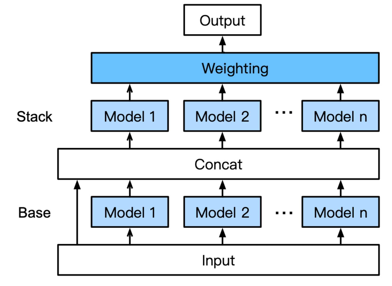
With .fit(train_df, presets="best_quality"), we are able to achieve 82/1692 in the competition. To reproduce our number, you may try the command mentioned in link.

Solar Radiation Prediction
In the second example, we will train model to predict the solar radiation. The orignal dataset is available in Kaggle Solar Radiation Prediction. The dataset contains such columns as: “wind direction”, “wind speed”, “humidity” and “temperature”. The response parameter that is to be predicted is: “Solar_radiation”. It contains measurements for the past 4 months and you have to predict the level of solar radiation. Let’s download and load the dataset.
!wget https://deep-earth.s3.amazonaws.com/datasets/earthcube2021_demo/SolarPrediction.csv.zip -O SolarPrediction.csv.zip
--2021-05-16 08:44:25--  https://deep-earth.s3.amazonaws.com/datasets/earthcube2021_demo/SolarPrediction.csv.zip
Resolving deep-earth.s3.amazonaws.com (deep-earth.s3.amazonaws.com)... 52.217.95.209
Connecting to deep-earth.s3.amazonaws.com (deep-earth.s3.amazonaws.com)|52.217.95.209|:443... connected.
HTTP request sent, awaiting response... 200 OK
Length: 523425 (511K) [application/zip]
Saving to: ‘SolarPrediction.csv.zip’

SolarPrediction.csv 100%[===================>] 511.16K  --.-KB/s    in 0.007s

2021-05-16 08:44:25 (76.8 MB/s) - ‘SolarPrediction.csv.zip’ saved [523425/523425]
import pandas as pd
df = pd.read_csv('SolarPrediction.csv.zip')
train_df, dev_df = train_test_split(df, random_state=100)
train_df.head(10)
| UNIXTime | Data | Time | Radiation | Temperature | Pressure | Humidity | WindDirection(Degrees) | Speed | TimeSunRise | TimeSunSet | |
|---|---|---|---|---|---|---|---|---|---|---|---|
| 2664 | 1474412104 | 9/20/2016 12:00:00 AM | 12:55:04 | 1039.15 | 65 | 30.40 | 57 | 2.26 | 5.62 | 06:11:00 | 18:21:00 |
| 12230 | 1476543319 | 10/15/2016 12:00:00 AM | 04:55:19 | 1.21 | 51 | 30.46 | 23 | 181.58 | 6.75 | 06:17:00 | 17:59:00 |
| 11706 | 1476704422 | 10/17/2016 12:00:00 AM | 01:40:22 | 1.22 | 50 | 30.47 | 39 | 142.56 | 10.12 | 06:18:00 | 17:58:00 |
| 12924 | 1476330025 | 10/12/2016 12:00:00 AM | 17:40:25 | 28.35 | 59 | 30.45 | 42 | 167.42 | 4.50 | 06:16:00 | 18:02:00 |
| 27507 | 1482367563 | 12/21/2016 12:00:00 AM | 14:46:03 | 637.93 | 57 | 30.39 | 74 | 40.94 | 4.50 | 06:53:00 | 17:49:00 |
| 2516 | 1474457405 | 9/21/2016 12:00:00 AM | 01:30:05 | 1.21 | 45 | 30.39 | 73 | 159.07 | 3.37 | 06:11:00 | 18:20:00 |
| 32227 | 1480723808 | 12/2/2016 12:00:00 AM | 14:10:08 | 177.19 | 45 | 30.34 | 93 | 134.78 | 11.25 | 06:42:00 | 17:42:00 |
| 12705 | 1476396922 | 10/13/2016 12:00:00 AM | 12:15:22 | 1008.08 | 65 | 30.46 | 46 | 71.24 | 5.62 | 06:17:00 | 18:01:00 |
| 14992 | 1475697322 | 10/5/2016 12:00:00 AM | 09:55:22 | 292.44 | 55 | 30.47 | 101 | 18.70 | 7.87 | 06:14:00 | 18:08:00 |
| 23615 | 1478267417 | 11/4/2016 12:00:00 AM | 03:50:17 | 1.18 | 44 | 30.42 | 38 | 176.34 | 7.87 | 06:25:00 | 17:47:00 |
Like in our previos example, we can directly train a predictor with a single .fit() call. The difference is that AutoGluon can automatically determine that it is a regression problem.
predictor = TabularPredictor(label='Radiation', eval_metric='r2', path='ag_ec2021_demo2').fit(train_df)
Warning: path already exists! This predictor may overwrite an existing predictor! path="ag_ec2021_demo2"
Beginning AutoGluon training ...
AutoGluon will save models to "ag_ec2021_demo2/"
AutoGluon Version:  0.2.1b20210511
Train Data Rows:    24514
Train Data Columns: 10
Preprocessing data ...
AutoGluon infers your prediction problem is: 'regression' (because dtype of label-column == float and many unique label-values observed).
	Label info (max, min, mean, stddev): (1601.26, 1.11, 206.52072, 315.54334)
	If 'regression' is not the correct problem_type, please manually specify the problem_type argument in fit() (You may specify problem_type as one of: ['binary', 'multiclass', 'regression'])
Using Feature Generators to preprocess the data ...
Fitting AutoMLPipelineFeatureGenerator...
	Available Memory:                    27858.63 MB
	Train Data (Original)  Memory Usage: 7.88 MB (0.0% of available memory)
	Inferring data type of each feature based on column values. Set feature_metadata_in to manually specify special dtypes of the features.
	Stage 1 Generators:
		Fitting AsTypeFeatureGenerator...
	Stage 2 Generators:
		Fitting FillNaFeatureGenerator...
	Stage 3 Generators:
		Fitting IdentityFeatureGenerator...
		Fitting DatetimeFeatureGenerator...
	Stage 4 Generators:
		Fitting DropUniqueFeatureGenerator...
	Types of features in original data (raw dtype, special dtypes):
		('float', [])                      : 3 | ['Pressure', 'WindDirection(Degrees)', 'Speed']
		('int', [])                        : 3 | ['UNIXTime', 'Temperature', 'Humidity']
		('object', ['datetime_as_object']) : 4 | ['Data', 'Time', 'TimeSunRise', 'TimeSunSet']
	Types of features in processed data (raw dtype, special dtypes):
		('float', [])                : 3 | ['Pressure', 'WindDirection(Degrees)', 'Speed']
		('int', [])                  : 3 | ['UNIXTime', 'Temperature', 'Humidity']
		('int', ['datetime_as_int']) : 4 | ['Data', 'Time', 'TimeSunRise', 'TimeSunSet']
	16.7s = Fit runtime
	10 features in original data used to generate 10 features in processed data.
	Train Data (Processed) Memory Usage: 1.96 MB (0.0% of available memory)
Data preprocessing and feature engineering runtime = 16.74s ...
AutoGluon will gauge predictive performance using evaluation metric: 'r2'
	To change this, specify the eval_metric argument of fit()
Automatically generating train/validation split with holdout_frac=0.1, Train Rows: 22062, Val Rows: 2452
Fitting 11 L1 models ...
Fitting model: KNeighborsUnif ...
	0.9501	 = Validation r2 score
	0.03s	 = Training runtime
	0.1s	 = Validation runtime
Fitting model: KNeighborsDist ...
	0.9531	 = Validation r2 score
	0.03s	 = Training runtime
	0.1s	 = Validation runtime
Fitting model: LightGBMXT ...
[1000]	train_set's l2: 5825	train_set's r2: 0.941343	valid_set's l2: 6881.24	valid_set's r2: 0.932405
[2000]	train_set's l2: 4818.35	train_set's r2: 0.951483	valid_set's l2: 6360.95	valid_set's r2: 0.937497
[3000]	train_set's l2: 4202.38	train_set's r2: 0.957684	valid_set's l2: 6212.24	valid_set's r2: 0.938993
[4000]	train_set's l2: 3751.34	train_set's r2: 0.962227	valid_set's l2: 6130.43	valid_set's r2: 0.939774
[5000]	train_set's l2: 3396.38	train_set's r2: 0.965805	valid_set's l2: 6110.98	valid_set's r2: 0.939962
[6000]	train_set's l2: 3117.1	train_set's r2: 0.968616	valid_set's l2: 6078.9	valid_set's r2: 0.940272
[7000]	train_set's l2: 2876.17	train_set's r2: 0.971039	valid_set's l2: 6073.82	valid_set's r2: 0.940339
[8000]	train_set's l2: 2666.91	train_set's r2: 0.973145	valid_set's l2: 6064.97	valid_set's r2: 0.940439
[9000]	train_set's l2: 2479.79	train_set's r2: 0.97503	valid_set's l2: 6082.82	valid_set's r2: 0.940253
	0.9405	 = Validation r2 score
	22.47s	 = Training runtime
	0.3s	 = Validation runtime
Fitting model: LightGBM ...
	0.9438	 = Validation r2 score
	2.37s	 = Training runtime
	0.02s	 = Validation runtime
Fitting model: RandomForestMSE ...
[1000] train_set's l2: 2247.86 train_set's r2: 0.977368 valid_set's l2: 5751.29 valid_set's r2: 0.943489
	0.9436	 = Validation r2 score
	6.91s	 = Training runtime
	0.1s	 = Validation runtime
Fitting model: CatBoost ...
	0.942	 = Validation r2 score
	4.38s	 = Training runtime
	0.0s	 = Validation runtime
Fitting model: ExtraTreesMSE ...
	0.9445	 = Validation r2 score
	2.1s	 = Training runtime
	0.1s	 = Validation runtime
Fitting model: NeuralNetFastAI ...
No improvement since epoch 0: early stopping
	-0.3674	 = Validation r2 score
	12.72s	 = Training runtime
	0.04s	 = Validation runtime
Fitting model: XGBoost ...
	0.9447	 = Validation r2 score
	5.8s	 = Training runtime
	0.01s	 = Validation runtime
Fitting model: NeuralNetMXNet ...
	0.9348	 = Validation r2 score
	77.28s	 = Training runtime
	0.12s	 = Validation runtime
Fitting model: LightGBMLarge ...
	0.9445	 = Validation r2 score
	12.47s	 = Training runtime
	0.01s	 = Validation runtime
Fitting model: WeightedEnsemble_L2 ...
	0.9547	 = Validation r2 score
	0.36s	 = Training runtime
	0.0s	 = Validation runtime
AutoGluon training complete, total runtime = 171.49s ...
TabularPredictor saved. To load, use: predictor = TabularPredictor.load("ag_ec2021_demo2/")
We can evaluate on the development set by calling .evaluate(). Here, we have specified the model to use R2 score so it will report the R2.
predictor.evaluate(dev_df)
Evaluation: r2 on test data: 0.9543093262635433
Evaluations on test data:
{
    "r2": 0.9543093262635433,
    "root_mean_squared_error": -67.7654685984138,
    "mean_squared_error": -4592.158734362603,
    "mean_absolute_error": -24.437721801314463,
    "pearsonr": 0.9768914212616937,
    "median_absolute_error": -1.0411042070388794
}
{'r2': 0.9543093262635433,
 'root_mean_squared_error': -67.7654685984138,
 'mean_squared_error': -4592.158734362603,
 'mean_absolute_error': -24.437721801314463,
 'pearsonr': 0.9768914212616937,
 'median_absolute_error': -1.0411042070388794}
Similarly, we can also measure the feature importance.
importance = predictor.feature_importance(dev_df)
importance
Computing feature importance via permutation shuffling for 10 features using 1000 rows with 3 shuffle sets...
	10.78s	= Expected runtime (3.59s per shuffle set)
	4.0s	= Actual runtime (Completed 3 of 3 shuffle sets)
| importance | stddev | p_value | n | p99_high | p99_low | |
|---|---|---|---|---|---|---|
| UNIXTime | 1.063341 | 0.042203 | 0.000262 | 3 | 1.305167 | 0.821515 |
| Time | 0.080480 | 0.004762 | 0.000583 | 3 | 0.107768 | 0.053192 |
| Temperature | 0.029517 | 0.001956 | 0.000730 | 3 | 0.040723 | 0.018311 |
| Data | 0.005320 | 0.001238 | 0.008781 | 3 | 0.012411 | -0.001771 |
| Humidity | 0.004958 | 0.000768 | 0.003948 | 3 | 0.009356 | 0.000560 |
| TimeSunRise | 0.003704 | 0.001029 | 0.012388 | 3 | 0.009599 | -0.002192 |
| TimeSunSet | 0.003685 | 0.001873 | 0.038180 | 3 | 0.014417 | -0.007047 |
| Pressure | 0.000460 | 0.000689 | 0.183299 | 3 | 0.004408 | -0.003487 |
| WindDirection(Degrees) | 0.000051 | 0.001093 | 0.471685 | 3 | 0.006313 | -0.006211 |
| Speed | 0.000006 | 0.000357 | 0.489087 | 3 | 0.002052 | -0.002039 |
More Information
You may check our website for more information and tutorials: https://auto.gluon.ai/. We also support automatically train models with text, image, and multimodal tabular data.
References
Erickson, Nick and Mueller, Jonas and Shirkov, Alexander and Zhang, Hang and Larroy, Pedro and Li, Mu and Smola, Alexander, AutoGluon-Tabular: Robust and Accurate AutoML for Structured Data, 2020, https://arxiv.org/pdf/2003.06505.pdf