OGGM-Edu - Jupyter notebooks to learn and teach about glaciers

Authors
Fabien Maussion, Erik Holmgren, Lindsey Nicholson, Lizz Ultee, Zora Schirmeister, Patrick Schmitt, Lilian Schuster
Author1 = {“name”: “Fabien Maussion”, “affiliation”: “University of Innsbruck”, “email”: “fabien.maussion@uibk.ac.at”, “orcid”: “https://orcid.org/0000-0002-3211-506X”}
Author2 = {“name”: “Erik Holmgren”, “affiliation”: “University of Innsbruck”, “email”: “erik.holmgren@student.uibk.ac.at”, “orcid”: “”}
Author3 = {“name”: “Lindsey Nicholson”, “affiliation”: “University of Innsbruck”, “email”: “lindsey.nicholson@uibk.ac.at”, “orcid”: “https://orcid.org/0000-0003-0430-7950”}
Author4 = {“name”: “Lizz Ultee”, “affiliation”: “Georgia Tech”, “email”: “eultee3@gatech.edu”, “orcid”: “https://orcid.org/0000-0002-8780-3089”}
Author5 = {“name”: “Zora Schirmeister”, “affiliation”: “University of Innsbruck”, “email”: “zora.schirmeister@student.uibk.ac.at”, “orcid”: “”}
Author6 = {“name”: “Patrick Schmitt”, “affiliation”: “University of Innsbruck”, “email”: “patrick.schmitt@student.uibk.ac.at”, “orcid”: “”}
Author7 = {“name”: “Lilian Schuster”, “affiliation”: “University of Innsbruck”, “email”: “lilian.schuster@student.uibk.ac.at”, “orcid”: “https://orcid.org/0000-0003-2101-2070”}
Table of Contents
- 1 OGGM-Edu - Jupyter notebooks to learn and teach about glaciers
- 2 Setup
- 3 Part 1: Idealized glacier experiments
- 4 Part 2: Real-world glacier experiments
- 4.1 Glaciers as water resources: idealized climate
- 4.2 Glaciers as water resources: projection with CMIP5
- 4.3 Part 2: Take home points
- 5 References
Purpose
OGGM-Edu (http://edu.oggm.org) is an educational platform providing instructors with tools that allow the demonstration of the governing principles of glacier behaviour. It offers online interactive apps and Jupyter notebooks that can be run in a browser via MyBinder or JupyterHub.
This notebook demonstrates how an open source numerical glacier model (OGGM) can be used to tackle scientific and socially-relevant research questions in class assignments and student projects. It is built on two independent numerical experiments:
the first section uses idealized glaciers (with controlled boundary conditions) to illustrate how climate and topography influence glacier behavior, and
the second section relies on realistic glaciers to illustrate how downstream freshwater resources will be affected by glacier change in the future.
The notebook contains code sections that serve as templates, followed by example research questions and suggestions that invite the student to re-run the experiment with updated simulation parameters. This notebook (as well as all other similar notebooks featured on the OGGM-Edu platform) is meant to be used and adapted by instructors to match the topics of a specific lecture or workshop. Interested readers will find more example notebooks on OGGM-Edu.
OGGM-Edu’s notebooks can help students to overcome barriers posed by numerical modelling and coding, in a fun, question-driven and societally relevant way.
Technical contributions
teach about fundamental concepts in glaciology in a modern, fun and interactive way
a numerical model used in research is used and abstracted (simplified) for teaching purposes
open and reproducible: the notebooks are all licensed with BSD3, and they can be run in openly available docker environments or on MyBinder
Methodology
The notebook relies on a number of standard packages of the scientific python ecosytem: NumPy, SciPy, xarray, pandas, etc. The main tool used for the modelling of glaciers is the Open Global Glacier Model (OGGM, http://oggm.org, https://docs.oggm.org). We also rely on a small number of helper functions (mostly to hide some of the OGGM internals to the readers) from the OGGM-Edu python package. For more details about OGGM-Edu, visit https://edu.oggm.org.
Results
The main outcome of this example notebook is a template, that can be used in glaciology workshops and classes. Example applications include a three-day workshop in Peru for university students without prior experience in glaciology (repository, more info) or the University of Michigan CLaSP 474 Ice and Climate notebooks.
Funding
Award1 = {“agency”: “University of Innsbruck”, “award_code”: “Förderkreis 1669 – Wissen schafft Gesell schaft”, “award_URL”: “https://www.uibk.ac.at/foerderkreis1669”}
Award2 = {“agency”: “Bundesministerium für Bildung und Forschung - BMBF”, “award_code”: “FKZ 01LS1602A”, “award_URL”: “https://www.bmbf.de”}
Keywords
keywords=[“glaciers”, “climate”, “education”, “python”, “numerical model”]
Citation
Maussion, F., Holmgren, E., Nicholson, L., Ultee, L., Schirmeister, Z., Schmitt, P., Schuster, L.. OGGM-Edu - Jupyter notebooks to learn and teach about glaciers. Jupyter Notebook accessed 11.06.2021 at https://github.com/OGGM/EarthCube2021
Suggested next steps
Visit https://edu.oggm.org and try the other notebooks there!
Setup
# import oggm-edu helper package
import oggm_edu as edu

# Plotting libraries and plot style
import matplotlib.pyplot as plt
%matplotlib inline

import seaborn as sns
sns.set_context('notebook')
sns.set_style('ticks')

# Scientific packages
import numpy as np
import pandas as pd
import xarray as xr

# OGGM flowline model
from oggm.core.flowline import RectangularBedFlowline

# OGGM mass-balance model
from oggm.core.massbalance import LinearMassBalance

# There are several numerical implementations in OGGM core. We use the "FluxBasedModel"
from oggm.core.flowline import FluxBasedModel as FlowlineModel
# Constants
import oggm.cfg
# Initialize OGGM and do not write on screen
oggm.cfg.initialize_minimal(logging_level='CRITICAL')
# Prevent numerical inaccuracies
oggm.cfg.PARAMS['cfl_number'] = 5e-3
# Store only the relevant variables here
oggm.cfg.PARAMS['store_diagnostic_variables'] = ['volume', 'area', 'length']
Part 1: Idealized glacier experiments
This part of the notebook shows how idealized glacier geometries can be used to explore basic principles of ice flow and glacier behavior.
This section is inspired from the OGGM-Edu notebooks “Glacier flowline modelling”, “Ice flow parameters” and “Mass-balance gradient”.
Glacier flowlines
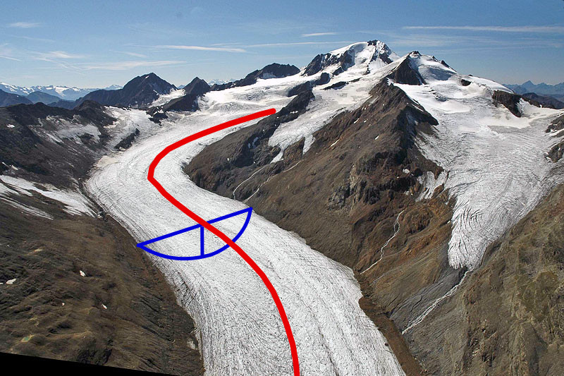
OGGM is a so-called flowline model, which means that the glacier ice flow is assumed to happen along a representative “1.5 dimensional” flowline, as in the image below. Why “1.5D” instead of 1 or 2? Although glacier ice can flow in only one direction along the flowline, each point of the glacier has a geometrical width, which can be different for different points. This means that 1.5D flowline models are able to match the observed area-elevation distribution of true glaciers, and can parametrize how glacier width changes with ice thickness change.
The first step for the experiment is now to define our idealized glacier geometry with OGGM:
# define horizontal resolution of the model:
# nx: number of grid points
# map_dx: grid point spacing in meters
nx = 200
map_dx = 100

# define glacier top and bottom altitudes in meters
top = 3400
bottom = 1400

# create a linear bedrock profile from top to bottom
bed_h, surface_h = edu.define_linear_bed(top, bottom, nx)

# glacier width in meters
initial_width = 600

# calculate the distance from the top to the bottom of the glacier in km
distance_along_glacier = edu.distance_along_glacier(nx, map_dx)

# Now describe the widths in units of "grid points" for the model, based on grid point spacing map_dx
widths = np.zeros(nx) + initial_width / map_dx

# Define our glacier flowine
init_flowline = RectangularBedFlowline(surface_h=surface_h, bed_h=bed_h, widths=widths, map_dx=map_dx)
We created the geometry of our glacier. It is very simple: ice will flow along a constant slope, and the glacier bed shape is constant as well (“U-shaped”, called rectangular in the model).
# plot the glacier bedrock profile and the initial glacier surface
plt.plot(distance_along_glacier, surface_h, label='Initial glacier')
edu.plot_xz_bed(x=distance_along_glacier, bed=bed_h);
The init_flowline object now contains all geometrical information needed by the model. It can give us access to some glacier attributes, which will be updated through the simulation:
print('Glacier length:', init_flowline.length_m)
print('Glacier area:', init_flowline.area_km2)
print('Glacier volume:', init_flowline.volume_km3)
Glacier mass balance
In this simple example, glaciers will gain mass via solid precipitation (snow/ice) and lose mass via melt. We will implement a glacier mass balance model to account for how much mass is gained or lost at each time step. To learn about mass-balance processes in more detail, visit our mass-balance notebook and this introduction to Glacier Mass Balance on AntarcticGlaciers.org.
We will use a simple linear function to describe the mass balance, defined by the equilibrium line altitude (ELA, the zone where annual accumulation - mass gain - and ablation - mass loss- are equal) and the gradient (mass-balance change with altitude, altgrad, unit [mm yr\(^{-1}\) m\(^{-1}\)]):
# ELA at 3000m a.s.l., gradient 4 mm yr-1 m-1
ELA = 3000  # equilibrium line altitude in meters above sea level
altgrad = 4  # altitude gradient in mm yr-1 m-1
mb_model = LinearMassBalance(ELA, grad=altgrad)
The OGGM mass-balance model computes the mass balance for any given altitude (unit: meters of ice per time [m s\(^{-1}\)], a simplification for the ice dynamics model). Let’s compute the annual mass balance along the glacier profile:
annual_mb = mb_model.get_annual_mb(surface_h) * oggm.cfg.SEC_IN_YEAR

# Plot it
plt.plot(annual_mb, bed_h, color='C2', label='Mass balance')
plt.xlabel('Annual mass balance (m yr-1)')
plt.ylabel('Altitude (m)')
plt.legend(loc='best')

# Display equilibrium line altitude, where annual mass balance = 0
plt.axvline(x=0, color='k', linestyle='--', linewidth=0.8)
plt.axhline(y=mb_model.ela_h, color='k', linestyle='--', linewidth=0.8);
plt.text(-7, ELA+30, 'ELA' );
These values are not too far from observed values of accumulation and melt in many regions of the world.
Independant research: can you find out what typical mass-balance gradient values can be measured on various glaciers of the world, and what climate variable(s) are the most relevant for them?
A first run
To let our glacier grow in various climate and topography conditions we need a glacier evolution model. A glacier evolution model is simply a combination of the initial bed topography (the flowline) and the climate (the mass-balance model). Let’s build it!
# The model requires the initial glacier bed, a mass-balance model, and an initial time (the year y0)
glacier_model = FlowlineModel(init_flowline, mb_model=mb_model, y0=0.)
# Let's run the model for a number of years (here 600), and store the output
_, ds = glacier_model.run_until_and_store(600)
The model output is stored in an xarray dataset. Fortunately, it makes exploring the output relatively easy:
Tip: click on the variables and the icons on the right to explore their attributes
ds
Now let’s plot the glacier attributes length, area and volume over time:
f, (ax1, ax2, ax3) = plt.subplots(1, 3, figsize=(18, 5))
ds.length_m.plot(ax=ax1);
ax1.set_xlabel('Years'); ax1.set_ylabel('Length (m)');
(ds.area_m2 * 1e-6) .plot(ax=ax2);
ax2.set_xlabel('Years'); ax2.set_ylabel('Area (km$^2$)');
(ds.volume_m3 * 1e-9) .plot(ax=ax3);
ax3.set_xlabel('Years'); ax3.set_ylabel('Volume (km$^3$)');
The first year of the simulation sees a big step increase in length and area: this is simply because the mass balance is positive at the top of the glacier, and we go from no glacier at all to a thin, but already 4 km long glacier. After this, the glacier constantly grows until reaching an equilibrium. This happens when the mass gain at the top of the glacier is compensated by mass loss at the tongue.
Do you see the small steps in length and area (specifically after the year 400)? This is because the length of a glacier in OGGM is defined by grid points of a specific grid size, i.e the step size.
What does a glacier at equilibrium look like? Let’s have a look:
# Get the glacier geometry at the end of the simulation
geometry = glacier_model.get_diagnostics()
The output of get_diagnostics() is a pandas data frame, which is very descriptive. We won’t have a look at all output variables today, but here is an overview:
geometry.head()
geometry.bed_h.plot(color='k', linestyle=':', label='Bedrock')
geometry.surface_h.plot(label='Glacier surface');
plt.legend(); plt.xlabel('Distance along flowline [m]'); plt.ylabel('Altitude [m]');
What does it mean when a glacier is in equilibrium with its climate? It means that its volume doesn’t change with time (which we can verify in the plots above), and that the total mass balance (averaged over the glacier area) is approximately equal to zero:
mb_model.get_specific_mb(fls=glacier_model.fls) # units of mm water equivalent per year
Close enough! We are in the following situation, where accumulation at the top compensates ablation at the bottom:
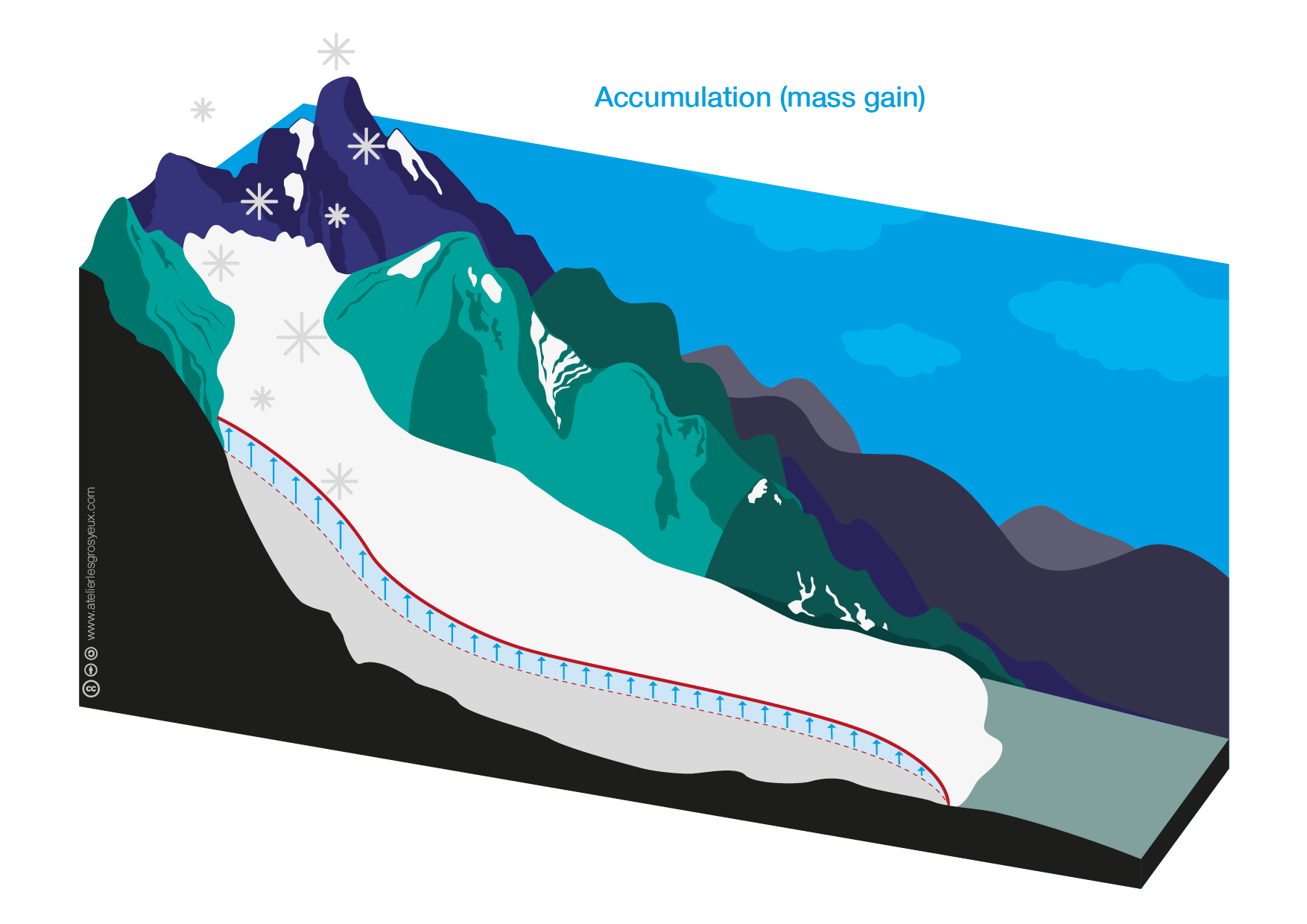
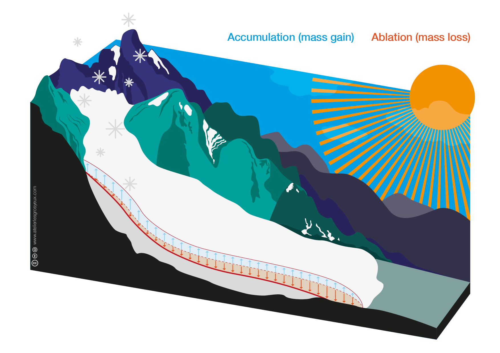
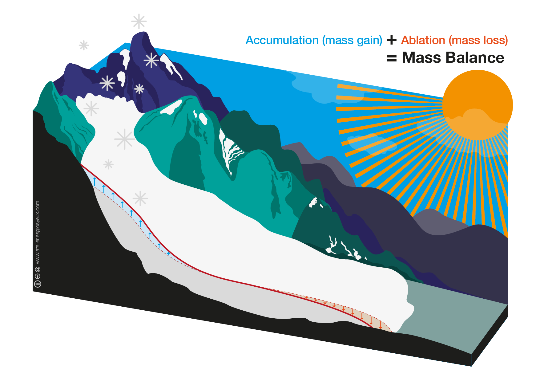
Source: OGGM-Edu’s open glacier graphics, made by Anne Maussion (Atelier les Gros yeux)
Now, a very common misconception is that a glacier which doesn’t advance or retreat also doesn’t move. We are going to show that our glacier is alive and well, and does move quite a lot even if it’s not growing or shrinking!
# plot the model glacier
plt.figure(figsize=(18, 5))
ax = plt.subplot(121)
velocity = geometry.ice_velocity * oggm.cfg.SEC_IN_YEAR
velocity.plot(ax=ax);
plt.legend(); plt.xlabel('Distance along flowline [m]'); plt.ylabel('Ice velocity [m yr$^{-1}$]');
plt.title('Ice velocity along the glacier (m yr$^{-1}$)');
plt.subplot(122)
edu.plot_glacier_graphics(num='06', title='Ice flow compensates for mass balance')
What is happening here? If enough ice piles up, it will move under the influence of gravity - very much like a fluid! At equilibrium, this ice flow compensates exactly for the mass gain (it removes ice at the top) and the mass loss (it replaces ice melt at the bottom).
A few meters per year is not enough for us to notice, but satellites can:
Source: FYFD
Experiment: Influence of the mass-balance gradient on glacier size
There are glaciers in many mountain areas of the world. To verify this yourself, we recommend spending a few minutes on the World Glacier Explorer, one of OGGM-Edu’s web applications.
In the app, we learned that glaciers can be located in maritime climates (regions with high amounts of precipitation and relatively warm) and in dry climates (rather dry and cold). These climate features can be translated to our simple framework by the mass-balance gradient:
A large mass-balance gradient represents high amounts of solid precipitation and high amounts of melt (maritime climate)
A small mass-balance gradient represents low amounts of solid precipitation and low amounts of melt (dry climate)
Now let’s translate this into our model code:
# Define the mass-balance gradients (MBG) we want to compare
# We will calculate models with the MBGs: 1, 4 and 15 mm yr-1 m-1.
# These values are realistic for real-world glaciers
gradients = [1, 4, 15]

# We use lists to store the output
mb_profiles = []
glacier_diagnostics = []
glacier_evolution = []

# equilibrium line altitude (ELA)
ELA = 3000

# Loop over the chosen gradients
for gradient in gradients:
    # Preparation of the mass-balance model for each gradient
    mb_model = LinearMassBalance(ELA, grad=gradient)

    # Run the simulation
    glacier_model = FlowlineModel(init_flowline, mb_model=mb_model, y0=0.)
    _, ds = glacier_model.run_until_and_store(1200)

    # Store the output for the plots later
    mb_profiles.append(mb_model.get_annual_mb(surface_h) * oggm.cfg.SEC_IN_YEAR)
    glacier_diagnostics.append(glacier_model.get_diagnostics())
    glacier_evolution.append(ds)

# Don't worry, this can take some time - but not more than one minute or two!
This time, we ran the model for 1200 years instead of 600 - we will get back to this soon. Let’s plot our glaciers first:
# Plot the results
f, (ax1, ax2) = plt.subplots(1, 2, figsize=[14, 6], sharey=True)

# Annual mass balance
ax = ax1
for gradient, profile in zip(gradients, mb_profiles):
    ax.plot(profile, bed_h, label='Mass balance, grad={}'.format(gradient))
# Add ELA, where mass balance = 0:
ax.axhline(y=ELA, color='k', linestyle='--', linewidth=0.8, label='Equilibrium line altitude')
ax.axvline(x=0, color='k', linestyle='--', linewidth=0.8)
ax.set_xlabel('Annual mass balance (m yr-1)'); ax.set_ylabel('Altitude (m)'); ax.legend(loc='best');

# Glacier profiles
ax = ax2
ax.plot(glacier_diagnostics[0].index, glacier_diagnostics[0].bed_h, color='k', label='Bedrock')
for gradient, diagnostics in zip(gradients, glacier_diagnostics):
    ax.plot(diagnostics.index, diagnostics.surface_h, label='Glacier surface, grad={}'.format(gradient));
ax.set_xlabel('Distance along flowline [m]'); ax.set_ylabel('Altitude [m]'); ax.legend(loc='best');
ax.axhline(y=ELA, color='k', linestyle='--', linewidth=0.8, label='Equilibrium line altitude');
Questions to address with an instructor or with independant research:
Visually check the amount of melt at the terminus of the glacier. Compare this with melt values you can find documented for real glaciers (for example, data from the World Glacier Monitoring Service or from scientific publications).
Why are all the glaciers symmetrical around the equilibrium line altitude? In the jargon, the ratio of the area above the equilibrium line altitude (ELA) divided by the entire area is called the Accumulation Area Ratio (AAR): here, it is 50%. Compare this with values you can find in the literature, and explain which of the assumptions we used can lead to this rather unusual AAR.
Now look at the top of the glacier in the accumulation area. Based on your observations, explain what the “mass-balance elevation feedback” might be, and what role it plays in our case.
Try to make a list of the mechanisms responsible for the different glacier sizes.
Tip: some definitions
Accumulation-area ratio (AAR): The ratio, often expressed as a percentage, of the area of the accumulation zone to the area of the glacier. The AAR is bounded between 0 and 1. On many glaciers it correlates well with the climatic mass balance. The likelihood that the climatic mass balance will be positive increases as the AAR approaches 1. (from the Glossary of glacier mass balance and related terms)
Mass-balance elevation feedback: a positive feedback which links ice elevation with mass balance. When ice thickens, its surface rises to higher elevations, which are colder and may receive more solid precipitation, hence thickening further. The same feedback also applies to the thinning case (“positive feedback” occurs when an inital perturbation is enhanced further by the feedback processes).
Bonus analysis: Temporal evolution of the glaciers
Now let’s plot the volume evolution of all three glaciers with time:
for gradient, ds in zip(gradients, glacier_evolution):
    (ds.volume_m3 * 1e-9).plot(label='Glacier volume, grad={}'.format(gradient));
plt.legend(); plt.xlabel('Years'); plt.ylabel('Volume (km$^3$)');
Questions to address:
Compare how long each glacier needs to reach equilibrium.
Why does one glacier respond much faster compared to another?
Now plot the ice velocity of all three glaciers at equilibrium. Discuss.
for gradient, geometry in zip(gradients, glacier_diagnostics):
    (geometry.ice_velocity * oggm.cfg.SEC_IN_YEAR).plot(label='Velocity, grad={}'.format(gradient));
plt.legend(); plt.xlabel('Distance along flowline [m]'); plt.ylabel('Ice velocity (m yr$^{-1}$)');
Exercise: Influence of glacier slope
Now repeat the analyses by varying another parameter: glacier slope.
Questions to address:
What is the influence of the glacier slope on how large the glacier will be in equilibrium and how fast the glacier responds. Can you explain this?
Plot the ice velocities. This might help to understand what happens.
For instructors: see the code below.
# Reset the mass-balance model to defaults. ELA at 3000m a.s.l., gradient 4 mm yr -1 m-1
ELA = 3000  # equilibrium line altitude in meters above sea level
altgrad = 4  # altitude gradient in mm/m
mb_model = LinearMassBalance(ELA, grad=altgrad)

# We use lists to store the output
mb_profiles = []
glacier_diagnostics = []
glacier_evolution = []

# To change the slope, we don't change anything to our bedrock parameters but the grid point resolution
factors = [0.7, 1, 1.5]
for factor in factors:
    # Define our glacier flowine
    init_flowline = RectangularBedFlowline(surface_h=surface_h, bed_h=bed_h, widths=widths, map_dx=map_dx * factor)
    # The glacier evolution model and the run
    glacier_model = FlowlineModel(init_flowline, mb_model=mb_model, y0=0.)

    # Run the simulation
    glacier_model = FlowlineModel(init_flowline, mb_model=mb_model, y0=0.)
    _, ds = glacier_model.run_until_and_store(1200)

    # Store the output for the plots later
    mb_profiles.append(mb_model.get_annual_mb(surface_h) * oggm.cfg.SEC_IN_YEAR)
    glacier_diagnostics.append(glacier_model.get_diagnostics())
    glacier_evolution.append(ds)
# Glacier profiles
f, ax = plt.subplots()
for factor, diagnostics in zip(factors, glacier_diagnostics):
    diagnostics.bed_h.plot(ax=ax, color='k', linestyle=':', label='')
    diagnostics.surface_h.plot(ax=ax, label='Glacier surface, factor={}'.format(factor));
ax.set_xlabel('Distance along flowline [m]'); ax.set_ylabel('Altitude [m]'); ax.legend(loc='best');
ax.axhline(y=ELA, color='k', linestyle='--', linewidth=0.8, label='Equilibrium line altitude');
for factor, ds in zip(factors, glacier_evolution):
    (ds.volume_m3 * 1e-9).plot(label='Glacier volume, factor={}'.format(factor));
plt.legend(); plt.xlabel('Years'); plt.ylabel('Volume (km$^3$)');
for factor, geometry in zip(factors, glacier_diagnostics):
    (geometry.ice_velocity * oggm.cfg.SEC_IN_YEAR).plot(label='Velocity, factor={}'.format(factor));
plt.legend(); plt.xlabel('Distance along flowline [m]'); plt.ylabel('Ice velocity (m yr$^{-1}$)');
More questions that could be asked:
What do you think are other factors that could influence how fast a glacier responds?
Repeat the analysis with the glacier length and compare it to the volume. What responds faster?
Part 2: Real-world glacier experiments
Part 1 explained how to use OGGM to answer theoretical questions about glaciers, using idealized experiments: the effect of a different slope, the concept of the equilibrium line altitude, the mass-balance gradient, etc. Now, how do we use OGGM to explore real glaciers? This section will give us some insights.
This section is inspired from the OGGM-Edu notebooks “Glaciers as water resources” part 1 and part 2.
Glaciers as water resources: idealized climate
Goals of this section:
Prepare a model run for a real world glacier.
Run simulations using different idealized climate scenarios to explore the role of glaciers as water resources.
Understand the concept of “peak water”.
Setting the scene: glacier runoff and “peak water”
“If glaciers melt, there won’t be water in the mountains anymore”.
This is a sentence that we often hear from people we meet, or sometimes even in news articles. In fact, the role of glaciers in the hydrological cycle is more complex than that. In this notebook, we will explore this question using idealized climate scenarios applied to real glaciers!
Before we continue, let’s have a look at the expected contribution of glaciers to local streamflow. The chart below shows an idealized scenario where first the climate is constant (t\(_0\)-t\(_1\)) and the glacier is in equilibrium with its climate. Then a warming occurs (t\(_1\)-t\(_2\)) and the glacier begins to lose mass. This graph makes a few very important points, which we will explore together in this notebook.
When a glacier is in equilibrium, it makes no net contribution to the annual runoff since the winter uptake of water, in the form of snow, is as large as the summer release through melt.
When the climate is warming, glaciers are losing mass. This water contributes to downstream runoff, and the runoff increases.
If climate warms even more, glaciers will continue to lose mass and become significantly smaller. When there isn’t much ice left to melt each summer (or when climate stabilizes), their contribution will become smaller, until it becomes zero again.
In the new equilibrium, the annual basin runoff is the same as before, but the seasonal pattern has changed.
We will now get back to all these points together, using OGGM!
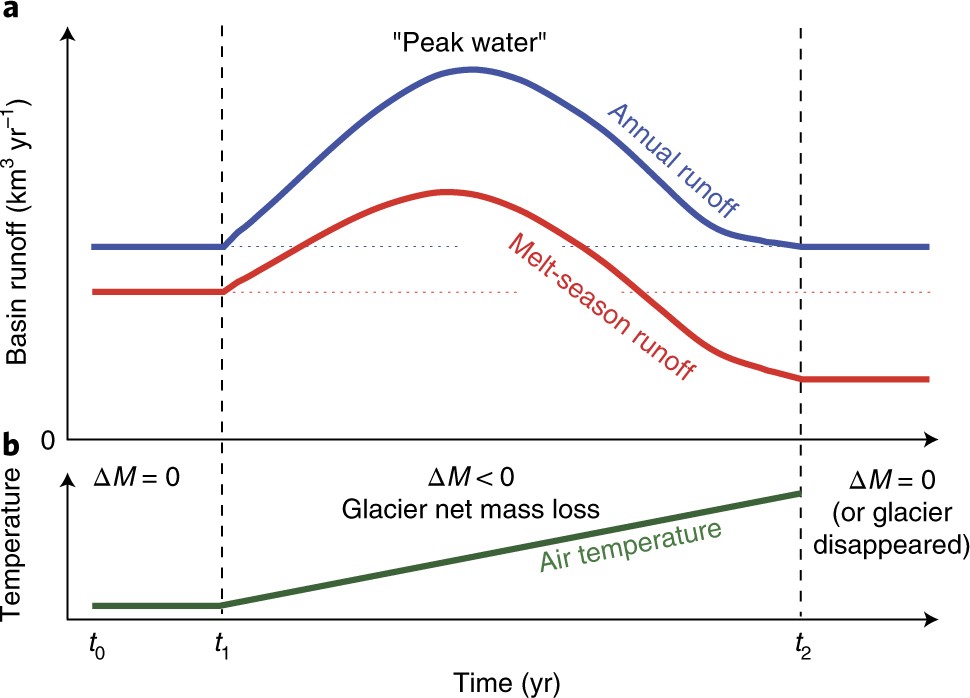
Graphic from Huss & Hock (2018)
Setup
# One interactive plot below requires Bokeh
# The rest of the notebook works without this dependency
import holoviews as hv
hv.extension('bokeh')
import geoviews as gv
import geoviews.tile_sources as gts
import salem
from oggm import utils, workflow, tasks, graphics
from oggm_edu import run_constant_climate_with_bias
# OGGM options
oggm.cfg.initialize(logging_level='WARNING')
oggm.cfg.PATHS['working_dir'] = utils.gettempdir(dirname='WaterResources')
oggm.cfg.PARAMS['min_ice_thick_for_length'] = 1  # a glacier is when ice thicker than 1m
Define the glacier we will play with
For this notebook we use the Hintereisferner, Austria. Some other possibilities to play with:
Hintereisferner, Austria: RGI60-11.00897
Artesonraju, Peru: RGI60-16.02444
Parlung No. 94, China: RGI60-15.11693
…and virtually any glacier you can find the RGI ID from (consult the GLIMS viewer for IDs)! Large glaciers may need longer simulations to see changes. For less uncertain model calibration parameters, we also recommend to pick one of the many reference glaciers listed here, where we make sure that observations of mass balance are better matched.
Let’s start with Hintereisferner first and you’ll be invited to try out your favorite glacier at the end of this notebook.
# Hintereisferner
rgi_id = 'RGI60-11.00897'
Importing preprocessed glacier data
Here we import all necessary data of the glacier. OGGM provides six different levels of preprocessed glacier directories. Each directory contains all the needed information for one glacier, like the geometry of the flowlines or the climate information for the mass-balance. For a detailed description of the different preprocessed levels you can look here and the raw data sources are listed here.
The import can take up to a few minutes on the first call because of the download of the required data:
# We pick the elevation-bands glaciers because they run a bit faster - but they create more step changes in the area outputs
base_url = 'https://cluster.klima.uni-bremen.de/~oggm/gdirs/oggm_v1.4/L3-L5_files/CRU/elev_bands/qc3/pcp2.5/no_match'
gdir = workflow.init_glacier_directories([rgi_id], from_prepro_level=5, prepro_border=80, prepro_base_url=base_url)[0]
Interactive glacier map
A first glimpse on the glacier of interest.
Tip: You can use the mouse to pan and zoom in the map
sh = salem.transform_geopandas(gdir.read_shapefile('outlines'))
(gv.Polygons(sh).opts(fill_color=None, color_index=None) * gts.tile_sources['EsriImagery'] *
 gts.tile_sources['StamenLabels']).opts(width=800, height=500, active_tools=['pan', 'wheel_zoom'])
As described above, glaciers in the OGGM world are “1.5 dimensional” along their flowline:
fls = gdir.read_pickle('model_flowlines')
graphics.plot_modeloutput_section(fls);
Generating a glacier in equilibrium with climate
Let’s prepare a run with the run_constant_climate_with_bias tasks from the oggm_edu package. It allows us to run idealized temperature and precipitation correction scenarios in an easy way.
First, let’s decide on a temperature evolution:
years = np.arange(400)
temp_bias_ts = pd.Series(years * 0. - 2, index=years)
temp_bias_ts.plot(); plt.xlabel('Year'); plt.ylabel('Temperature bias (°C)');
Not much to see here! The temp_bias_ts variable describes a temperature bias that will be applied to the standard climate (see below).
Here the bias is -2° all along because we want to run a so-called “spinup” run, to let the glacier grow and make sure that our glacier is in dynamical equilibrium with its climate at the end of the simulation. Let’s go:
# file identifier where the model output is saved
file_id = '_spinup'

# We are using the task run_with_hydro to store hydrological outputs along with the usual glaciological outputs
tasks.run_with_hydro(gdir,  # Run on the selected glacier
                     temp_bias_ts=temp_bias_ts,  # the temperature bias to apply to the average climate
                     run_task=run_constant_climate_with_bias,  # which climate scenario? See below for more examples
                     y0=2009, halfsize=10,  # Period which we will average and constantly repeat
                     store_monthly_hydro=True,  # Monthly ouptuts provide additional information
                     output_filesuffix=file_id);  # an identifier for the output file, to read it later
OK, so there is quite some new material in the cell above. Let’s focus on the most important points:
We run the model for 400 years (as defined by our control temperature time series)
The model runs with a constant climate based on the average over 21 years (2 times
halfsize+ 1) for the period 1999-2019We apply a cold bias of -2°C. Indeed, Hintereisferner is in strong disequilibrium with the current climate and this cold bias is needed to make the glacier grow (more on this later)
Let’s have a look at the output now:
with xr.open_dataset(gdir.get_filepath('model_diagnostics', filesuffix=file_id)) as ds:
    # The last step of hydrological output is NaN (we can't compute it for this year)
    ds = ds.isel(time=slice(0, -1)).load()
There are plenty of variables in this dataset! We can list them with:
ds
Tip: you can click on a variable and show its attribute with the “page” button on the right.
The time and month_2d variables are coordinates, and the other variables are either provided as additional information (e.g. calendar_month, we will get back to this), or they are providing the actual data. For instance, we can plot the annual evolution of the volume and length of our glacier:
fig, axs = plt.subplots(nrows=2, figsize=(10, 7), sharex=True)
ds.volume_m3.plot(ax=axs[0]);
ds.length_m.plot(ax=axs[1]);
axs[0].set_xlabel(''); axs[0].set_title(f'{rgi_id}'); axs[1].set_xlabel('Years');
The glacier grows and almost doubles its volume. After 400 years, it is in equilibrium.
This spinup simulation won’t be analyzed further: let’s jump to the heart of the topic: what happens with glacier runoff when climate is warming?
Climate change simulation
We start by generating a temperature change scenario. We define a short period of constant temperature (at -2°C, to be consistent with above), followed by a linear increase (2.5 degrees in about 150 years) and a stabilization:
ny_s = 50  # Start
ny_t = 150  # Trend
ny_e = 102  # Stabilisation
temp_bias_ts = np.concatenate([np.full(ny_s, -2.), np.linspace(-2, 0.5, ny_t), np.full(ny_e, 0.5)])
temp_bias_ts = pd.Series(temp_bias_ts, index=np.arange(ny_s + ny_t + ny_e))
temp_bias_ts.plot(); plt.xlabel('Year'); plt.ylabel('Temperature bias (°C)');
# file identifier where the model output is saved
file_id = '_lin_temp'

# We are using the task run_with_hydro to store hydrological outputs along with the usual glaciological outputs
tasks.run_with_hydro(gdir,
                     temp_bias_ts=temp_bias_ts,  # the temperature bias timeseries we just created
                     run_task=run_constant_climate_with_bias,  # which climate scenario? See following notebook for other examples
                     y0=2009, halfsize=10,  # Period which we will average and constantly repeat
                     store_monthly_hydro=True,  # Monthly ouptuts provide additional information
                     init_model_filesuffix='_spinup',  # We want to start from the glacier in equibrium we created earlier
                     output_filesuffix=file_id);  # an identifier for the output file, to read it later
Let’s have a look at our glacier evolution:
with xr.open_dataset(gdir.get_filepath('model_diagnostics', filesuffix=file_id)) as ds:
    # The last step of hydrological output is NaN (we can't compute it for this year)
    ds = ds.isel(time=slice(0, -1)).load()
fig, axs = plt.subplots(nrows=3, figsize=(10, 7), sharex=True)
ds.volume_m3.plot(ax=axs[0]);
ds.length_m.plot(ax=axs[1]);
temp_bias_ts.plot(ax=axs[2], c='C3');
axs[0].set_xlabel(''); axs[0].set_title(f'{rgi_id}'); axs[1].set_xlabel(''); axs[2].set_xlabel('Years'); axs[2].set_ylabel('Temperature bias (°C)');
In this scenario, the glacier would melt almost entirely (it loses about 90% of its volume). Note also that the glacier continues to adjust after the temperature has stabilized.
What are the implications for downstream runoff?
Annual runoff
As glaciers retreat, they contribute to sea-level rise (visit the World Glaciers Explorer OGGM-Edu app for more information!). This is however not what we are interested in for this notebook. Instead we will explore an important local impact of glaciers: their impact on streamflow.
Let’s take a look at some of the hydrological outputs computed by OGGM. We start by creating a pandas DataFrame of all “1D” (annual) variables in the output dataset:
sel_vars = [v for v in ds.variables if 'month_2d' not in ds[v].dims]
df_annual = ds[sel_vars].to_dataframe()
Then we can select the hydrological variables and sum them to get the total annual runoff:
Note that we convert the annual runoff from kilos to mega-tonnes (Mt)
# Select only the runoff variables
runoff_vars = ['melt_off_glacier', 'melt_on_glacier', 'liq_prcp_off_glacier', 'liq_prcp_on_glacier']
# Convert them to megatonnes (instead of kg)
df_runoff = df_annual[runoff_vars] * 1e-9
# We smooth the output, which is otherwize noisy because of area discretization
df_runoff = df_runoff.rolling(31, center=True, min_periods=1).mean()
fig, ax = plt.subplots(figsize=(10, 3.5), sharex=True)
df_runoff.sum(axis=1).plot(ax=ax);
plt.ylabel('Runoff (Mt)'); plt.xlabel('Years'); plt.title(f'Total annual runoff for {rgi_id}');
The hydrological variables are computed on the largest possible area that was covered by glacier ice during the simulation. This is equivalent to the runoff that would be measured at a fixed-gauge hydrological station at the glacier terminus.
The total annual runoff consists of the following components:
Melt off-glacier: snow melt on areas that are now glacier free (i.e. 0 in the year of largest glacier extent, in this example at the start of the simulation)
Melt on-glacier: ice + seasonal snow melt on the glacier
Liquid precipitation on- and off-glacier (the latter being zero at the year of largest glacial extent, in this example at the start of the simulation)
f, ax = plt.subplots(figsize=(10, 6));
df_runoff.plot.area(ax=ax, color=sns.color_palette('rocket')); plt.xlabel('Years');
plt.ylabel('Runoff (Mt)'); plt.title(rgi_id);
The glacier length and volume decrease from year 50 onwards until about year 250 - this is the glacier retreat phase. Afterwards, length and volume stabilize at a constant value indicating that the glacier has reached equilibrium.
Now study the graph above and it’s four main components.
Questions to address:
When is “peak water” reached? Does this have anything to do with a change in the temperature trend itself? If not, what is the reason for “peak water” to occur?
Verify that the total fixed-gauge runoff (remember what this means?) is the same at the beginning and the end of the simulation. Why is that so? What changed in between?
The temperature stabilizes at year 200, yet all hydrological variables continue to change after that. What is happening there?
What is the contribution of liquid precipitation at the beginning and the end of the simulation? What changed?
Can you verify that the net glacier contribution to runoff (i.e. - \(\Delta M / \Delta t\) is zero at the beginning and the end of the simulation and positive in between? Why do we expect this behavior?
Hint: compare the results to the idealised runoff graphic that we introduced at the beginning of this chapter
# Solution of the last question above
glacier_mass = ds.volume_m3.to_series() * oggm.cfg.PARAMS['ice_density'] * 1e-9  # In Megatonnes, Mt
glacier_mass = glacier_mass.rolling(31, center=True, min_periods=1).mean()
(- glacier_mass.diff()).plot()
plt.axhline(y=0, color='k', ls=':')
plt.ylabel('Annual glacier mass change (Mt yr$^{-1}$)')
plt.xlabel('Years'); plt.title('Glacier contribution to annual runoff');
Monthly runoff
The “2D” variables contain the same hydrological data, but at monthly resolution (dimensions [time, month]). For example, monthly runoff can be computed as:
# Select only the runoff variables and convert them to megatonnes (instead of kg)
monthly_runoff = (ds['melt_off_glacier_monthly'] + ds['melt_on_glacier_monthly'] +
                  ds['liq_prcp_off_glacier_monthly'] + ds['liq_prcp_on_glacier_monthly'])
monthly_runoff = monthly_runoff.rolling(time=31, center=True, min_periods=1).mean() * 1e-9
monthly_runoff.clip(0).plot(cmap='Blues', cbar_kwargs={'label': 'Runoff (Mt)'}); plt.xlabel('Months'); plt.ylabel('Years');
But be aware, something is a bit wrong with this plot (some of you may have noticed: maximum melt happens in the fall, which is unusual). That’s because the OGGM coordinates are hydrological months - a side effect of using a so called mass balance year (or water year), which begins in October and ends in September (i.e. encompasses the entire accumulation and ablation season).
We have to correct for this by shifting the months forward:
# This should work in both hemispheres maybe?
ds_roll = ds.roll(month_2d=ds['calendar_month_2d'].data[0] - 1, roll_coords=True)
ds_roll['month_2d'] = ds_roll['calendar_month_2d']

# Select only the runoff variables and convert them to megatonnes (instead of kg)
monthly_runoff = (ds_roll['melt_off_glacier_monthly'] + ds_roll['melt_on_glacier_monthly'] +
                  ds_roll['liq_prcp_off_glacier_monthly'] + ds_roll['liq_prcp_on_glacier_monthly'])
monthly_runoff = monthly_runoff.rolling(time=31, center=True, min_periods=1).mean() * 1e-9
monthly_runoff.clip(0).plot(cmap='Blues', cbar_kwargs={'label': 'Runoff (Mt)'}); plt.xlabel('Months'); plt.ylabel('Years');
As we can see, the runoff is approximately zero during the winter months, while relatively high during the summer months.
Now let’s compare the actual runoff to total precipitation over the basin:
# Compute total precipitation (Snow + Liquid)
tot_precip = (ds_roll['liq_prcp_off_glacier_monthly'] + ds_roll['liq_prcp_on_glacier_monthly'] +
              ds_roll['snowfall_off_glacier_monthly'] + ds_roll['snowfall_on_glacier_monthly'])
tot_precip *= 1e-9  # in Mt
# Plot these data at year 0
yr = 0
r = monthly_runoff.sel(time=yr)
p = tot_precip.sel(time=yr)

f, ax = plt.subplots(figsize=(10, 6));
r.plot(ax=ax, color='C3', label='Monthly runoff', linewidth=3);
p.plot(ax=ax, color='C0', label='Monthly precipitation', linewidth=3);
ax.fill_between(r.month_2d, r, p, where=(p >= r), facecolor='C0', interpolate=True, alpha=0.5)
ax.fill_between(r.month_2d, r, p, where=(r > p), facecolor='C3', interpolate=True, alpha=0.5)
plt.ylabel('Mt yr$^{-1}$'); plt.legend(loc='best');
plt.xlabel('Month'); plt.title(f'Total monthly runoff and precipitation at year {yr}');
At the beginning of the simulation, the glacier is in equilibrium and its annual contribution to runoff is zero. In fact, this means that the blue area in the plot above is equal to the red area: the glaciated basin releases water during the summer, that accumulated in form of snow in the winter months.
In this region (Ötztal Alps, Austria), precipitation is relatively constant throughout the year. Discuss what the implications could be in other climates of the world, in particular in climates with a strong seasonality of precipitation.
Now let’s have a look at the seasonal change in runoff with time:
f, ax = plt.subplots(figsize=(10, 6));
cmap = sns.color_palette('magma', 3)
for i, yr in enumerate([0, 120, 300]):
    monthly_runoff.sel(time=yr).plot(ax=ax, color=cmap[i], label=f'Year {yr}')
plt.ylabel('Mt yr$^{-1}$'); plt.legend(loc='best');
plt.xlabel('Month'); plt.title('Total monthly runoff change with time');
Questions to explore:
Verify that the annual runoff is the same at year 0 than at year 300. What changed in between?
What is responsible for the switch from summer melt to spring melt?
How does the runoff change at “peak water” (approx. year 120)?
Discuss the implications of this shift in seasonality for Hintereisferner and for other regions of the world.
Now repeat this notebook (ideally by copying it first) with other regions of the world, where climate might be very different.
Note that the hydrological interpretation is very glacier-specific. So if you change the glacier by using another rgi_id, you also might need to adapt the notebook explanation in teaching!
You can also change the parameters of the simulations!
What happens when the temperature change is larger/faster, smaller/slower? What are the implications for “peak water”?
Wrapping up
Now let’s conclude this notebook by reproducing now this famous plot by Huss & Hock (2018) with our data.
Graphic from Huss & Hock (2018)
# Make a dataframe out of the xarray dataset for simplicity
df_monthly_runoff = pd.DataFrame(monthly_runoff.data, index=ds.time, columns=monthly_runoff.month_2d)

# Create new columns for each season (we define seasons from the perspective of the northern Hemisphere)
df_monthly_runoff['Spring (Apr-Jun)'] = df_monthly_runoff[[4, 5, 6]].sum(axis=1)
df_monthly_runoff['Summer (Jul-Sep)'] = df_monthly_runoff[[7, 8, 9]].sum(axis=1)
df_monthly_runoff['Winter (Oct-Mar)'] = df_monthly_runoff[[10, 11, 12, 1, 2, 3]].sum(axis=1)
df_monthly_runoff.columns.name = 'Season'

# Plot it
# Attention the seasons and labels might need to be adapted if a glacier in a different region is used!
f, ax = plt.subplots(figsize=(10, 6));
df_monthly_runoff[['Spring (Apr-Jun)', 'Summer (Jul-Sep)', 'Winter (Oct-Mar)']].plot.area(ax=ax, color=sns.color_palette('rocket'));
plt.xlabel('Years'); plt.ylabel('Runoff (Mt)'); plt.title('Runoff by season');
And now the actual plot:
f, (ax1, ax2) = plt.subplots(2, 1, gridspec_kw={'height_ratios': [2, 1]}, figsize=(10, 8), sharex=True)

p1 = df_monthly_runoff[['Spring (Apr-Jun)', 'Summer (Jul-Sep)', 'Winter (Oct-Mar)']].sum(axis=1)
p2 = df_monthly_runoff['Summer (Jul-Sep)'] # July to September is here the melt season
p1.plot(ax=ax1, color='C0', label='Annual runoff', linewidth=3)
p2.plot(ax=ax1, color='C3', label='Melt-season runoff', linewidth=3);
ax1.hlines([p1.loc[0], p2.loc[0]], 0, 300, color=['C0', 'C3'], linestyle=[':']);
ax1.legend(); ax1.set_xlabel(''); ax1.set_ylabel('Runoff (Mt)');

(temp_bias_ts + 2).plot(ax=ax2, color='C2', label='Temperature', linewidth=3);
ax2.legend(loc='lower right'); ax2.set_xlabel('Years'); ax2.set_ylabel('$\Delta T (°C)$');
sns.despine();
Note that the two plots above are very glacier-specific. If you use a glacier with another climate, you might need to adapt the plots, because we are always interested in those months where the runoff from the glacier contributes most to the total runoff. Example given, for Artesonraju in Peru, we are most interested in June, July, August and September as this is the dry season, where it almost does not rain at all.
Glaciers as water resources: projection with CMIP5
You have now learned how to simulate and analyse a specific glacier under an idealized climate. We will now take this a step further and simulate two different glaciers, located in different climatic regions, forced with CMIP5 (Coupled Model Intercomparison Project 5) climate projections.
We begin by initializing the glacier directories:
# We keep Hintereisferner from earlier, but also add a new glacier
rgi_ids = [rgi_id, 'RGI60-15.02420']
gdirs = workflow.init_glacier_directories(rgi_ids, from_prepro_level=5, prepro_border=80, prepro_base_url=base_url)
gdirs now contain two glaciers, one in Central Europe and one in the Eastern Himlayas:
gdirs
We can take a quick look at the new glacier:
sh = salem.transform_geopandas(gdirs[1].read_shapefile('outlines'))
(gv.Polygons(sh).opts(fill_color=None, color_index=None) * gts.tile_sources['EsriImagery'] *
 gts.tile_sources['StamenLabels']).opts(width=800, height=500, active_tools=['pan', 'wheel_zoom'])
Climate downscaling
Before we run our simulation we have to process the climate data for the glacier i.e. we downscale it: (This can take some time)
from oggm.shop import gcm_climate
bp = 'https://cluster.klima.uni-bremen.de/~oggm/cmip5-ng/pr/pr_mon_CCSM4_{}_r1i1p1_g025.nc'
bt = 'https://cluster.klima.uni-bremen.de/~oggm/cmip5-ng/tas/tas_mon_CCSM4_{}_r1i1p1_g025.nc'
for rcp in ['rcp26', 'rcp45', 'rcp60', 'rcp85']:
    # Download the files
    ft = utils.file_downloader(bt.format(rcp))
    fp = utils.file_downloader(bp.format(rcp))
    workflow.execute_entity_task(gcm_climate.process_cmip_data, gdirs,
                                 # Name file to recognize it later
                                 filesuffix='_CCSM4_{}'.format(rcp),
                                 # temperature projections
                                 fpath_temp=ft,
                                 # precip projections
                                 fpath_precip=fp,
                                 );
Projection run
With the downscaling complete, we can run the forced simulations:
for rcp in ['rcp26', 'rcp45', 'rcp60', 'rcp85']:
    rid = '_CCSM4_{}'.format(rcp)
    workflow.execute_entity_task(tasks.run_with_hydro, gdirs,
                                 run_task=tasks.run_from_climate_data, ys=2020,
                                 # use gcm_data, not climate_historical
                                 climate_filename='gcm_data',
                                 # use the chosen scenario
                                 climate_input_filesuffix=rid,
                                 # this is important! Start from 2020 glacier
                                 init_model_filesuffix='_historical',
                                 # recognize the run for later
                                 output_filesuffix=rid,
                                 # add monthly diagnostics
                                 store_monthly_hydro=True);
# Create the figure
f, ax = plt.subplots(figsize=(18, 7), sharex=True)
# Loop over all scenarios
for i, rcp in enumerate(['rcp26', 'rcp45', 'rcp60', 'rcp85']):
    file_id = f'_CCSM4_{rcp}'
    # Open the data, gdirs[0] correspond to Hintereisferner.
    with xr.open_dataset(gdirs[0].get_filepath('model_diagnostics', filesuffix=file_id)) as ds:
        # Load the data into a dataframe
        ds = ds.isel(time=slice(0, -1)).load()

    # Select annual variables
    sel_vars = [v for v in ds.variables if 'month_2d' not in ds[v].dims]
    # And create a dataframe
    df_annual = ds[sel_vars].to_dataframe()

    # Select the variables relevant for runoff.
    runoff_vars = ['melt_off_glacier', 'melt_on_glacier', 'liq_prcp_off_glacier', 'liq_prcp_on_glacier']
    # Convert to mega tonnes instead of kg.
    df_runoff = df_annual[runoff_vars].clip(0) * 1e-9
    # Sum the variables each year "axis=1", take the 11 year rolling mean
    # and plot it.
    df_runoff.sum(axis=1).rolling(window=11).mean().plot(ax=ax, label=rcp, color=sns.color_palette("rocket")[i])

ax.set_ylabel('Annual runoff (Mt)'); ax.set_xlabel('Year'); plt.title(rgi_id); plt.legend();
For Hintereisferner, runoff continues to decrease throughout the 21st-century for all scenarios, indicating that “peak water” has already been reached sometime in the past. This is the case for many European glaciers. What about our unnamed glacier in the Himalayas?
# Create the figure
f, ax = plt.subplots(figsize=(18, 7), sharex=True)
# Loop over all scenarios
for i, rcp in enumerate(['rcp26', 'rcp45', 'rcp60', 'rcp85']):
    file_id = f'_CCSM4_{rcp}'
    # Open the data, gdirs[1] correspond to the unnamed glacier.
    with xr.open_dataset(gdirs[1].get_filepath('model_diagnostics', filesuffix=file_id)) as ds:
        # Load the data into a dataframe
        ds = ds.isel(time=slice(0, -1)).load()

    # Select annual variables
    sel_vars = [v for v in ds.variables if 'month_2d' not in ds[v].dims]
    # And create a dataframe
    df_annual = ds[sel_vars].to_dataframe()

    # Select the variables relevant for runoff.
    runoff_vars = ['melt_off_glacier', 'melt_on_glacier',
                   'liq_prcp_off_glacier', 'liq_prcp_on_glacier']
    # Convert to mega tonnes instead of kg.
    df_runoff = df_annual[runoff_vars].clip(0) * 1e-9
    # Sum the variables each year "axis=1", take the 11 year rolling mean
    # and plot it.
    df_runoff.sum(axis=1).rolling(window=11).mean().plot(ax=ax, label=rcp, color=sns.color_palette("rocket")[i])

ax.set_ylabel('Annual runoff (Mt)'); ax.set_xlabel('Year'); plt.title(gdirs[1].rgi_id); plt.legend();
Unlike for Hintereisferner, these projections indicate that the annual runoff will increase in all the scenarios for the first half of the century. The higher RCP scenarios can reach “peak water” later in the century, since the excess melt can continue to increase. For the lower RCP scenarios on the other hand, the glacier might be approaching a new equilibrium, which reduces the runoff earlier in the century (Rounce et. al., 2020). After “peak water” is reached (RCP2.6: ~2055, RCP8.5: ~2070 in these projections), the annual runoff begins to decrease. This decrease occurs because the shrinking glacier is no longer able to support the high levels of melt.
Part 2: Take home points
Glaciers in equilibrium are not net water resources: they gain as much mass as they release over a year.
However, they have a seasonal buffer role: they release water during the melt months.
The size of a glacier has an influence on the water availability downstream during the dry season. The impact is most important if the (warm) melt season coincides with the dry season (see Kaser et al., 2010).
When glaciers melt, they become net water resources over the year. “Peak water” is the point in time when glacier melt supply reaches its maximum, i.e. when the maximum runoff occurs.
References
Scientific publications and books
Cuffey, K., and W. S. B. Paterson (2010). The Physics of Glaciers, Butterworth‐Heinemann, Oxford, U.K.
Huss, M. and Hock, R.: Global-scale hydrological response to future glacier mass loss, Nat. Clim. Chang., 8(2), 135–140, doi:10.1038/s41558-017-0049-x, 2018.
Kaser, G., Großhauser, M., and Marzeion, B.: Contribution potential of glaciers to water availability in different climate regimes, PNAS, 07 (47) 20223-20227, doi:10.1073/pnas.1008162107, 2010
Marzeion, B., Kaser, G., Maussion, F. and Champollion, N.: Limited influence of climate change mitigation on short-term glacier mass loss, Nat. Clim. Chang., 8, doi:10.1038/s41558-018-0093-1, 2018.
Rasmussen, L. A., & Andreassen, L. M. (2005). Seasonal mass-balance gradients in Norway. Journal of Glaciology, 51(175), 601-606.
Rounce, D. R., Hock, R., McNabb, R. W., Millan, R., Sommer, C., Braun, M. H., Malz, P., Maussion, F., Mouginot, J., Seehaus, T. C. and Shean, D. E.: Distributed global debris thickness estimates reveal debris significantly impacts glacier mass balance, Geophys. Res. Lett., doi:10.1029/2020GL091311, 2021.
Oerlemans, J. (2001). Glaciers and climate change. CRC Press.
Online books and articles
An EGU CryoBlog post about the role of glaciers in the hydrological cycle
AntarcticGlaciers.org: a fantastic resource to learn about glaciers.