.ipynb .pdf

Contents

Toward autonomous detection of anomalous GNSS data via applied unsupervised artificial intelligence

Unsupervised Anomaly Detection of TZVOLCANO GNSS Data using Gaussian Mixtures. Once loaded in Binder, please run all the cells to properly initialize values and GUI elements.

Authors

Mike Dye, D. Sarah Stamps, Myles Mason

• Author1 = {“name”: “Mike Dye”, “affiliation”: “Unaffiliated”, “email”: “mike@mikedye.com”, “orcid”: “0000-0003-2065-870X”}

• Author2 = {“name”: “Dr. Sarah Stamps”, “affiliation”: “Virginia Tech”, “email”: “dstamps@vt.edu”, “orcid”: “0000-0002-3531-1752”}

• Author3 = {“name”: “Myles Mason”, “affiliation”: “Virginia Tech”, “email”: “mylesm18@vt.edu”, “orcid”: “0000-0002-8811-8294”}

Table of Contents

• 1  Toward autonomous detection of anomalous GNSS data via applied unsupervised artificial intelligence
  • 1.1  Authors
  • 1.2  Purpose
  • 1.3  Technical contributions
  • 1.4  Methodology
  • 1.5  Results
  • 1.6  Funding
  • 1.7  Keywords
  • 1.8  Citation
  • 1.9  Suggested next steps
  • 1.10  Acknowledgements
  • 1.11  License
  • 1.12  Glossary
• 2  Setup
  • 2.1  Library import
  • 2.2  Local library import
• 3  Parameter definitions
• 4  Data import
  • • 4.0.1  Important note on imported data
  • 4.1  Select the instrument ID and the start and end date of the data to be processed and analyzed
  • 4.2  Select data file for use during analysis
  • 4.3  Read contents of the selected file in to a pandas object
• 5  Data processing and analysis
  • 5.1  Resample the data to fill in holes in the time series
    • 5.1.1  Make a copy of the unmodified data
    • 5.1.2  Alternative method: Make a copy of unmodified data and resample the time series to fill in any missing time values in the series
  • 5.2  Rescale the Features
  • 5.3  Calculate the Vector Magnitude
  • 5.4  Plot the Features
  • 5.5  Identify outliers for each feature with the Gaussian Mixtures algorithm
    • 5.5.1  Find outliers for the Scaled Height feature
    • 5.5.2  Find outliers for the Scaled Latitude feature
    • 5.5.3  Find outliers for the Scaled Longitude feature
    • 5.5.4  Find outliers for the Vector Magnitude feature
    • 5.5.5  Consolidate the arrays of times to remove in to one object
    • 5.5.6  Create a new pandas object with the points identified by the algorithm removed
    • 5.5.7  Plot the "cleaned" data on top of the original data
  • 5.6  Identify anomalies for each feature using the K-means algorithm
    • 5.6.1  find outliers for the Scaled Height feature
    • 5.6.2  find outliers for the Scaled Latitude feature
    • 5.6.3  find outliers for the Scaled Longitude feature
    • 5.6.4  find outliers for the Vector Magnitude feature
  • 5.7  Training the neural net
    • 5.7.1  Training on unfiltered data
      • 5.7.1.1  Generate the training set
      • 5.7.1.2  Create and train the neural network model
      • 5.7.1.3  Use the trained model to make prediction for N_STEPS_AHEAD time increments
    • 5.7.2  Training on data filtered using Gaussian Mixtures
      • 5.7.2.1  Generate the training set
      • 5.7.2.2  Create and train the neural network model
      • 5.7.2.3  Use the trained model to make prediction for N_STEPS_AHEAD time increments
    • 5.7.3  Training on data filtered using K-Means
      • 5.7.3.1  Generate the training set
      • 5.7.3.2  #### Create and train the neural network model
      • 5.7.3.3  Use the trained model to make prediction for N_STEPS_AHEAD time increments
    • 5.7.4  Plots of unfiltered data
    • 5.7.5  Plots of Gaussian Mixtures cleaned / filtered data
    • 5.7.6  Plots of K-means cleaned / filtered data
  • 5.8  Compare the accuracy of the prediction made by the different trained models
    • 5.8.1  The MSE of the unmodified data
    • 5.8.2  The MSE of the Gaussian Mixtures cleaned data
    • 5.8.3  The MSE of the K-Means cleaned data
    • 5.8.4  Percent improvement in neural network predictions
• 6  References

Purpose

This notebook demonstrates a process by which GNSS data (lontitude, latitude, and height) obtained from the TZVOLCANO CHORDS portal (Stamps et al., 2016) can be analyzed with minimal human input to remove data points that are manifestations of high noise, instrumentation error, and other factors that introduce large errors into specific measurements. These prepared and cleaned data are then used to train a neural network that can be used for detecting volcanic activity.

This notebook takes advantage of the Earthcube funded CHORDS infrastructure (Daniels et al., 2016; Kerkez et al., 2016), which powers the TZVOLCANO CHORDS portal. GNSS positioning data (longitude, latitude, and height) are from the active Ol Doinyo Lengai volcano in Tanzania, which are made available through UNAVCO’s real-time GNSS data services. UNAVCO’s real-time GNSS data services provides real-time positions processed by the Trimble Pivot system. Real-time GNSS data from several instruments are streamed into the TZVOLCANO portal using brokering scripts developed by Joshua Robert Jones in Python and D. Sarah Stamps in awk, which makes them instantly available via the CHORDS data API service.

Technical contributions

• Created a python-based API client to download data from a CHORDS portal

• Development of local libraries to download, manipulate, and plot GNSS data (longitude, latitude, and height) obtained from a CHORDS portal that obtains positions from UNAVCO’s real-time GNSS data services

• Identification and removal of statistical outliers in GNSS time-series data using the Gaussian Mixtures Algorithm

• Identification and removal of statistical outliers in GNSS time-series data using the K-means Algorithm

• Implementation of a neural net model which, when trained on these data, can make predictions based on the historical time series

Methodology

• Select instrument and date range of positioning data (longitude, latitude, and height) to analyze

• Download selected data set from TZVOLCANO CHORDS portal

• Scale and impute data to prepare them for machine learning algorithms

• Use a Gaussian Mixtures and then a K-means algorithm to identify and remove data points likely to have significant noise from each feature/variable

• Train three Neural networks: one using the unfiltered data and two using the “cleaned” data output from the Gaussian mixtures and K-Means algorithm

• Use predictions made by the these neural nets to make predictions (forecasts) of future data points

• Compare these predictions to actual values from the unmodified data set to quantify the reduction in noise achieved by the filtering algorithm

Results

Compared to the neural net trained on the unfiltered data, filtered (or “cleaned”) data output Machine Learning Visualizations (Gaussian Mixtures and K-means) result in trained neural net models that do a significantly better job of generating predictions.

Funding

The development of this notebook was not directly supported by any awards, however the notebook leverages the EarthCube cyberinfrastructure CHORDS which was funded by the National Science Foundation.

• Award1 = {“agency”: “US National Science Foundation”, “award_code”: “1440133”, “award_URL”: “https://www.nsf.gov/awardsearch/showAward?AWD_ID=1440133&HistoricalAwards=false”}

• Award2 = {“agency”: “US National Science Foundation”, “award_code”: “1639750”, “award_URL”: “https://www.nsf.gov/awardsearch/showAward?AWD_ID=1639750&HistoricalAwards=false”}

• Award3 = {“agency”: “US National Science Foundation”, “award_code”: “1639554”, “award_URL”: “https://www.nsf.gov/awardsearch/showAward?AWD_ID=1639554&HistoricalAwards=false”}

Keywords

keywords=[“TZVOLCANO”, “CHORDS”, “UNAVCO”, “Artificial Intelligence”, “Machine Learning”]

Citation

Dye, Mike, D. Sarah Stamps, Myles Mason (2021), Jupyter Notebook: Toward autonomous detection of anomalous GNSS data via applied unsupervised artificial intelligence, EarthCube Annual Meeting 2021

Suggested next steps

• A Support Vector Machine should be investigated as a possible filtering mechanism.

• CHORDS API should be made more robust and flexible.

• Predictions from the improved trained neural net model should be compared in real-time to incoming GNSS data to attempt to identify emerging volcanic events.

• Test if filtering data with both the Gaussian Mixtures and K-means in combination would further improve the neural net predictions.

• Use this same filtering process on time-series data from other CHORDS portals.

• Update citation with doi

• Investigate and compare the approach used in this notebook with benchmarks from classical time series filtering and prediction *

* As suggested by anonymous reviewer

Acknowledgements

• CHORDS: for providing a versatile and practical cyber-infrastructure component

• Virginia Tech: for enabling an incredibly supportive cutting edge learning and research environment

• EarthCube & Earthcube Office: for creating the opportunity to create and share notebook and creating a well-designed Jupyter notebook template

• Abbi Devins-Suresh: for testing this notebook and invaluable feedback

License

This notebook is licensed under the MIT License.

Glossary

A brief definition of these terms is provided below for terms that may be unfamiliar to those without experience with machine learning, or are used in ways that may be unusual or ambiguous.

• [Feature](https://en.wikipedia.org/wiki/Feature_(machine_learning): “a individual property or characteristic of a phenomenon being observed” (Wikipedia contributors, 2021). In this notebook, the imported fields (Time, Height, Longitude, and Latitude) are the initial features. One additional feature is calculated on the fly - the vector magnitude of scaled values of the original fields.

• Impute: In machine learning, the replacement of null or missing values with an actual value in order to facilitate processing by an algorithm.

• Anomaly: Data that for varying reasons do not occur within the usual ranges. In this notebook, there are (at least) two types of anomalies that may occur: those due to inaccurate measurements and subsequent processing, and those due to actual volcanic events.

Setup

Library import

# System functionality
import os
from pathlib import Path
from datetime import datetime

# Python ≥3.5 is required
import sys
assert sys.version_info >= (3, 5)

# Data manipulation
import numpy as np
import pandas as pd

# Plotting and Visualizations
%matplotlib inline
import matplotlib as mpl
import matplotlib.pyplot as plt

mpl.rc('axes', labelsize=14)
mpl.rc('xtick', labelsize=12)
mpl.rc('ytick', labelsize=12)

# Data pipeline, scaling, normalizing, etc
from sklearn.pipeline import Pipeline
from sklearn import preprocessing
from sklearn.preprocessing import StandardScaler
from sklearn.impute import SimpleImputer

# MSE calculation
from sklearn.metrics import mean_squared_error

# Machine Learning Algorithms
from sklearn.cluster import KMeans
from sklearn.mixture import GaussianMixture

# Neural Network Support

# Scikit-Learn ≥0.20 is required
import sklearn
assert sklearn.__version__ >= "0.20"

try:
    # %tensorflow_version only exists in Colab.
    %tensorflow_version 2.x
    IS_COLAB = True
except Exception:
    IS_COLAB = False
    
# TensorFlow ≥2.0 is required
import tensorflow as tf
from tensorflow import keras
assert tf.__version__ >= "2.0"

if not tf.config.list_physical_devices('GPU'):
    print("No GPU was detected. LSTMs and CNNs can be very slow without a GPU.")
    if IS_COLAB:
        print("Go to Runtime > Change runtime and select a GPU hardware accelerator.")

No GPU was detected. LSTMs and CNNs can be very slow without a GPU.

# Autoreload extension
if 'autoreload' not in get_ipython().extension_manager.loaded:
    %load_ext autoreload
    
%autoreload 2

# to make this notebook's output stable across runs
np.random.seed(42)
tf.random.set_seed(42)

Local library import

#####
# Function definitions are included in this file to improve code readability 
# 
# Many of these functions are based on code from the excellent book
# Hands-On Machine Learning with Scikit-Learn, Keras, and TensorFlow, 2nd Edition
# by Aurélien Géron
#####

# Include local library paths
sys.path.append('./libraries')

# Import local libraries

# Misc. functions to support data analysis
from TZVOLCANO_utilities import *
from TZVOLCANO_plotting import *
from TZVOLCANO_gaussian_mixtures import *
from TZVOLCANO_kmeans import *
from TZVOLCANO_neural_net import *

# CHORDS GUI interface (uses ChordsAPI.py)
from chords_gui import chords_gui 

Parameter definitions

# Initialize the CHORDS GUI and load the API. DOMAIN is the URL of your CHORDS portal. 
DOMAIN = 'tzvolcano.chordsrt.com'
CHORDS = chords_gui(DOMAIN)

# Define the initial start and end date for the date selector
INITIAL_START_DATE = '2021-01-01'
INITIAL_END_DATE = '2021-01-01'


# Min/max values used to scale the height, lon, and lat
# This should be either -1, 1 or 0, 1
SCALE_MINIMUM = 0
SCALE_MAXIMUM = 1

#####
# Define important parameters that control the neural net functionality.
#####
N_STEPS_TRAINING = 6 * 1000      # The number of data points to use in the training set
N_STEPS_FORECAST = 500           # The number of data points to display in the predictions graph
N_STEPS_AHEAD = 100              # the number of steps ahead that the neural net will predict


# Gaussian Mixtures Parameters
N_COMPONENTS = 1                 # The number of regions to generate - needs to be 1 for this use case
N_INIT = 10                      
COVARIANCE_TYPE = "tied"

Data import

Data for this notebook is stored in the TZVOLCANO CHORDS portal. In order to run the notebook, users will need to select a date range, an instrument identifier, and click the “Download File” button. The designated data file is then downloaded to the local server and can be selected for use.

The data is CSV format and is downloaded using the CHORDS API.

Each row of data includes a time, latitude, longitude, and height of instruments deployed on the Ol Doinyo Lengai volcano for the TZVOLCANO initiative. Below is a map of the instrument IDs to the TZVOLCANO designators:

Instrument ID    Instrument Name    Notes
1                OLO1               Live instrument
2                OLO3               Live instrument
4                OLOT               Test instrument with data from station BILL_RTX
5                OLO6               Live instrument
6                OLO7               Live instrument
7                OLO8               Live instrument
8                OLOJ               Test instrument 
9                OLON               Test instrument

The default for the notebook is to use OLO1 (instrument id 1). OLOT (instrument id 4) is a test site that contains data from station BILL_RTX. Data from other instruments may not be available for the default time window.

The default start and end dates are both set to January 1, 2021.

Important note on imported data

The entire date range is analyzed using the K-Means and the Gaussian Mixtures clustering identification algorithms.

The large number of data points (millions of points) would, however, slow the training of the neural networks to an unusable pace when running on a server without GPU support (such as the servers used by mybinder).

The N_STEPS_TRAINING parameter limits the number of data points fed to the neural network. 5,000 - 10,000 points seems to provide enough training data to make passable predictions and is still a small enough data set that training the net takes a reasonable amount of time (several minutes).

Select the instrument ID and the start and end date of the data to be processed and analyzed

The cell below must be run in order to display the CHORDS GUI!

CHORDS.start_end_widgets(INITIAL_START_DATE, INITIAL_END_DATE)

# Make sure that at least the default data file has been downloaded
number_of_data_files_found = len(CHORDS.get_availiable_files())
if (number_of_data_files_found < 1):
    CHORDS.download_csv_file()

Select data file for use during analysis

Choose which of the downloaded CSV files to use for analysis.

These files are retained on the server running the notebook indefinitely.

Note that on shared servers (such as mybinder.org) very large files may not work properly if they consume all available disk space and or memory

The cell below must be run in order to display the data file selection widget!

CHORDS.select_data_file()

Available Data Files

Read contents of the selected file in to a pandas object

if (CHORDS.available_data_files.value == None):
    print("no files were found")

file_name = CHORDS.available_data_files.value
print("Imported csv data from" + file_name)

unmodified_data = CHORDS.load_data_from_file(file_name)

Imported csv data fromtzvolcano_chordsrt_com_instrument_id_1_2021-01-01_to_2021-01-01.csv
csv_files/tzvolcano_chordsrt_com_instrument_id_1_2021-01-01_to_2021-01-01.csv

Data processing and analysis

Resample the data to fill in holes in the time series

Make a copy of the unmodified data

# Fill in missing points in the time series
resampled_data = unmodified_data.copy()

# Set the 'Time' field to be used as the index
resampled_data = resampled_data.set_index('Time').sort_index()

# Re-insert the 'Time' field, as changing it to be the index removes is as a referenceable field in the pandas object
resampled_data['Time'] = resampled_data.index

Alternative method: Make a copy of unmodified data and resample the time series to fill in any missing time values in the series

The standard approach for anomaly detection recommends imputing missing data points in a time-series. However, in this case the imputing approach was found to reduce the final accuracy of the predictions made by the neural network. The code below is commented out and is not executed. It was retained as documentation in case the imputing approach is helpful for other applications of this overall methodology.

# Make a copy of the unmodified data
# resampled_data = unmodified_data.copy()

# Fill in missing points in the time-series, inserting any times missing from the series using NaN as the value
# resampled_data = resampled_data.set_index('Time').sort_index().resample('1000ms').ffill()

# Re-insert the 'Time' field, as the resampling process changed it to be the index
# resampled_data['Time'] = resampled_data.index

Rescale the Features

Many clustering algorithms are highly sensitive to min-max ranges - including both the K-means and Gaussian mixtures algorithms. Here a best practice is followed, and before running the clustering algorithms, the data are rescaled.

Details of the scaling procedure can be found by examining the scale_np_data function.

# Rescale Height, Longitude and Latitude to the range between SCALE_MINIMUM and SCALE_MAXIMUM
scaled_data = pd.DataFrame()

# Convert the Time variable to Seconds Since Epoch
scaled_data["Seconds Since Epoch"] = resampled_data['Time'].astype(np.int64)
# scaled_data["Time"] = resampled_data['Time']

scaled_data["Scaled Height"] = scale_np_data(resampled_data["Height"].to_numpy(), SCALE_MINIMUM, SCALE_MAXIMUM)
scaled_data["Scaled Latitude"] = scale_np_data(resampled_data["Latitude"].to_numpy(), SCALE_MINIMUM, SCALE_MAXIMUM)
scaled_data["Scaled Longitude"] = scale_np_data(resampled_data["Longitude"].to_numpy(), SCALE_MINIMUM, SCALE_MAXIMUM)

Calculate the Vector Magnitude

Treating the individual fields as a vector, calculate the vector magnitude value as a derived feature.

Creating an derived feature (variable) is a common technique in machine learning. It often makes it possible to more easily detect patterns in correlated features. In this case, it makes it easier to identify regions of localized high-noise areas within the time series.

fields_list = ['Scaled Height', 'Scaled Latitude', 'Scaled Longitude']

scaled_data["Vector Magnitude"] = calculate_vector_magnitude(scaled_data, fields_list, SCALE_MINIMUM, SCALE_MAXIMUM)

Plot the Features

Note the “Vector Magnitude” feature in green. It’s wide range of values makes it easier for the algorithms to identify outliers.

plt.figure(figsize=(16, 10))

ax = plt.gca() # get current axis
alpha = 0.6

scaled_data.plot(kind='line',x='Seconds Since Epoch',y='Scaled Height', color='blue',ax=ax, alpha=alpha)
scaled_data.plot(kind='line',x='Seconds Since Epoch',y='Scaled Latitude', color='red', ax=ax, alpha=alpha)
scaled_data.plot(kind='line',x='Seconds Since Epoch',y='Scaled Longitude', color='orange', ax=ax, alpha=alpha)
scaled_data.plot(kind='line',x='Seconds Since Epoch',y='Vector Magnitude', color='green', ax=ax, alpha=alpha)
plt.show()

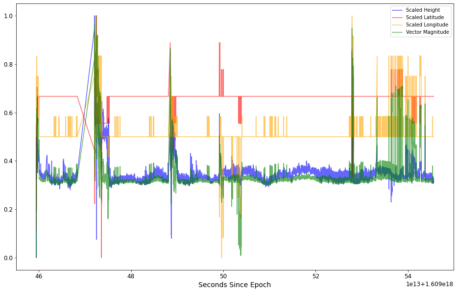
Note in the plot above, the Vector Magnitude feature in green. The wide range of values should make it easier for the clustering algorithms to identify areas of high noise within the signal.

Identify outliers for each feature with the Gaussian Mixtures algorithm

In order to save space and make the code more readable, several steps in this process have been abstracted out to functions in an external library.

For each feature, the same processing and analysis is applied:

• Designate which feature the is being used

• Designate a density threshold percent that determines the percentage of data point that will be classified as being outliers

• Perform transformations which scale and impute the data (see note) for the designated feature

• Train a Gaussian Mixtures model with the imputed data

• Generate a plot showing which points are flagged for removal

A manual part of this process is performed at this point: Determining what value of the density threshold percent yields the best results. The values that appear in this code were arrived at by executing this process, looking at the generated plot, adjusting the density threshold percent, and then re-running this section of the code. This was performed until the plot indicates that outliers are identified, and that points that should be retained are not flagged for removal.

Note: Imputing the data fills in missing values with the most frequently occurring value for that variable. This is necessary as the algorithm cannot function with missing values for times in the series.

Find outliers for the Scaled Height feature

field_name = 'Scaled Height'
scaled_height_density_threshold_percent = 5.2

scaled_height_data_imputed = transform_data_for_gaussian_mixtures(scaled_data, field_name)

scaled_height_gm, scaled_height_anomalies = get_anomalies_using_gaussian_mixtures(scaled_height_data_imputed, scaled_height_density_threshold_percent)

plot_gaussian_mixture_anomalies(scaled_height_gm, scaled_height_data_imputed, scaled_height_anomalies)

./libraries/TZVOLCANO_plotting.py:103: UserWarning: No contour levels were found within the data range.
  linewidths=2, colors='r', linestyles='dashed')

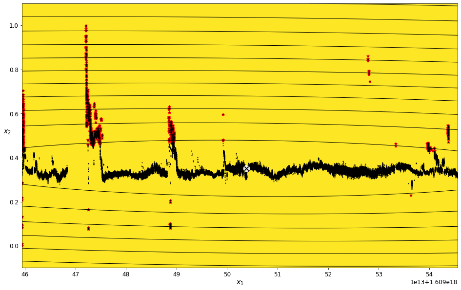
The red highlights in the plot above indicate the data points identified as being outside of the assigned density threshold. These are the points that will be removed in the data filtering and cleaning process.

Find outliers for the Scaled Latitude feature

field_name = 'Scaled Latitude'
scaled_latitude_density_threshold_percent = 3

scaled_latitude_data_imputed = transform_data_for_gaussian_mixtures(scaled_data, field_name)

scaled_latitude_gm, scaled_latitude_anomalies = get_anomalies_using_gaussian_mixtures(scaled_latitude_data_imputed, scaled_latitude_density_threshold_percent)

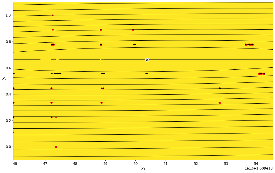
plot_gaussian_mixture_anomalies(scaled_latitude_gm, scaled_latitude_data_imputed, scaled_latitude_anomalies)

./libraries/TZVOLCANO_plotting.py:103: UserWarning: No contour levels were found within the data range.
  linewidths=2, colors='r', linestyles='dashed')

Find outliers for the Scaled Longitude feature

field_name = 'Scaled Longitude'
scaled_longitude_density_threshold_percent = 7

scaled_longitude_data_imputed = transform_data_for_gaussian_mixtures(scaled_data, field_name)

scaled_longitude_gm, scaled_longitude_anomalies = get_anomalies_using_gaussian_mixtures(scaled_longitude_data_imputed, scaled_longitude_density_threshold_percent)

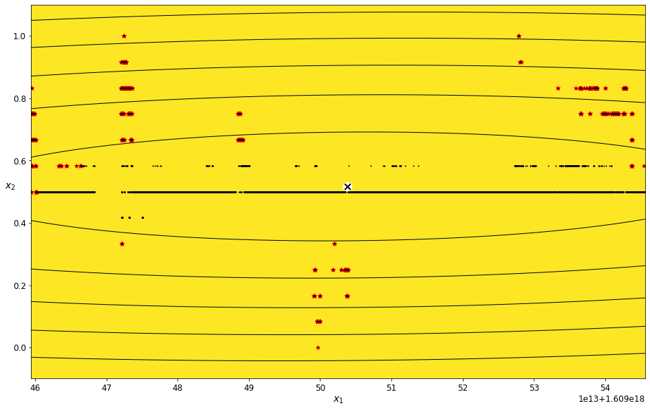
plot_gaussian_mixture_anomalies(scaled_longitude_gm, scaled_longitude_data_imputed, scaled_longitude_anomalies)

./libraries/TZVOLCANO_plotting.py:103: UserWarning: No contour levels were found within the data range.
  linewidths=2, colors='r', linestyles='dashed')

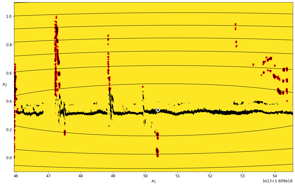
Find outliers for the Vector Magnitude feature

field_name = 'Vector Magnitude'
vector_magnitude_density_threshold_percent = 7

vector_magnitude_data_imputed = transform_data_for_gaussian_mixtures(scaled_data, field_name)

vector_magnitude_gm, vector_magnitude_anomalies = get_anomalies_using_gaussian_mixtures(vector_magnitude_data_imputed, vector_magnitude_density_threshold_percent)

plot_gaussian_mixture_anomalies(vector_magnitude_gm, vector_magnitude_data_imputed, vector_magnitude_anomalies)

./libraries/TZVOLCANO_plotting.py:103: UserWarning: No contour levels were found within the data range.
  linewidths=2, colors='r', linestyles='dashed')

Consolidate the arrays of times to remove in to one object

# convert the list of anomalies to datetime data type so they can be used to filter the scaled data set
scaled_height_times_to_remove    = pd.to_datetime(scaled_height_anomalies[:, 0], unit='ns', utc=True)
scaled_longitude_times_to_remove = pd.to_datetime(scaled_longitude_anomalies[:, 0], unit='ns', utc=True)
scaled_latitude_times_to_remove  = pd.to_datetime(scaled_latitude_anomalies[:, 0], unit='ns', utc=True)
vector_magnitude_times_to_remove = pd.to_datetime(vector_magnitude_anomalies[:, 0], unit='ns', utc=True)


# Consolidate the arrays of times to remove in to one object
times_to_remove = scaled_height_times_to_remove
times_to_remove = times_to_remove.union(scaled_longitude_times_to_remove)
times_to_remove = times_to_remove.union(scaled_latitude_times_to_remove)
times_to_remove = times_to_remove.union(vector_magnitude_times_to_remove)
times_to_remove = times_to_remove.drop_duplicates()

Create a new pandas object with the points identified by the algorithm removed

# remove the flagged times from the scaled data set 
g_m_cleaned_data = scaled_data.copy()
g_m_cleaned_data = g_m_cleaned_data.drop(times_to_remove)

Plot the “cleaned” data on top of the original data

plt.figure(figsize=(16, 10))

# get current axis
ax = plt.gca()
alpha = 0.99


scaled_data.plot(kind='line',x='Seconds Since Epoch',y='Vector Magnitude', color='blue',ax=ax, alpha=alpha)
g_m_cleaned_data.plot(kind='line',x='Seconds Since Epoch',y='Vector Magnitude', color='red',ax=ax, alpha=alpha)
ax.legend(["Vector Magnitude (Unfiltered) ", "Vector Magnitude (Filtered using Gaussian Mixtures)"]);
plt.show()

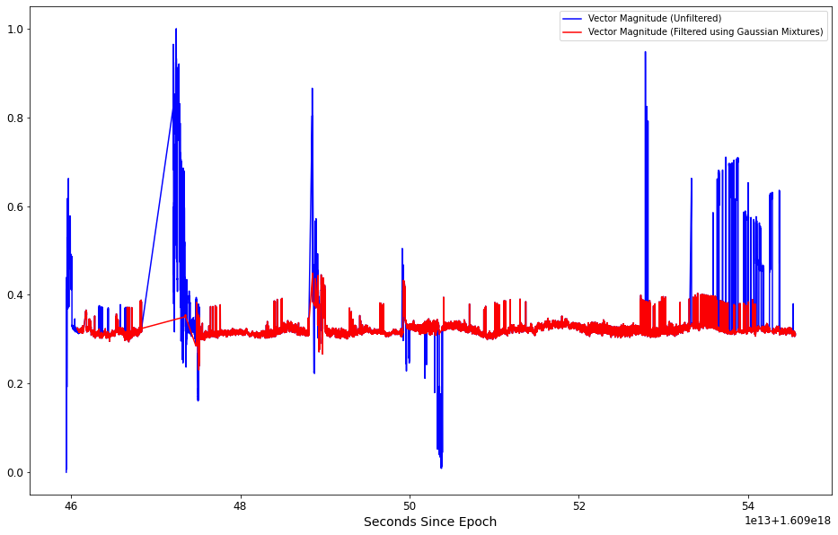
The plot above shows that the value ranges of the filtered data is much less than seen in the unmodified data. This is a good indicator that training a machine learning algorithm (such as a neural net) should result in a trained algorithm that produces more accurate predictions than if it were to be trained using the unfiltered data.

Identify anomalies for each feature using the K-means algorithm

find outliers for the Scaled Height feature

field_to_analyze = 'Scaled Height'
number_of_clusters = 10

# Impute the data 
scaled_height_kmeans_data_imputed = transform_data_for_kmeans(scaled_data, field_to_analyze)

# Train the K-means model
scaled_height_kmeans = KMeans(n_clusters=number_of_clusters, random_state=42)

scaled_height_cluster_labels = scaled_height_kmeans.fit_predict(scaled_height_kmeans_data_imputed)

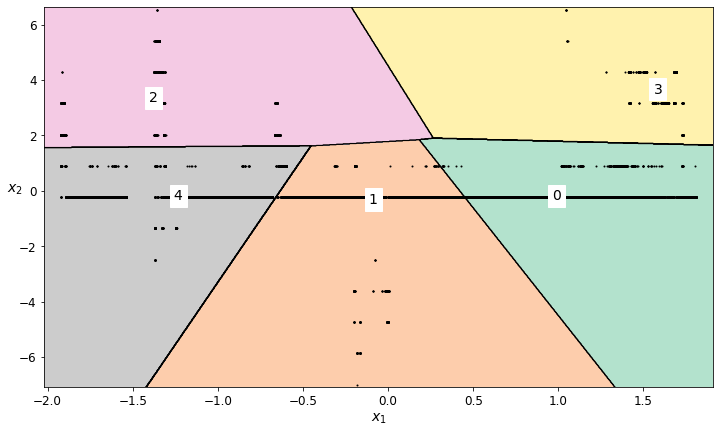
# Plot the decision boundaries
plt.figure(figsize=(12, 7))
plot_decision_boundaries(scaled_height_kmeans, scaled_height_kmeans_data_imputed)

The plot above shows the regions generated by the K-means algorithm. The numbers indicate the index of the associated region.

Some of the regions for this particular K-means plot is a bit messy, yet it can still be used to identify regions in the data that likely contain high noise and should be removed.

# Based on the labeled regions from the decision boundary plot, decide which regions should be retained
scaled_height_regions_to_retain = [4,1,5,3,0,8]

find outliers for the Scaled Latitude feature

# Generate a K-means cluster 
field_to_analyze = 'Scaled Latitude'
number_of_clusters = 5

# Impute and scale the data 
scaled_latitude_kmeans_imputed_data = transform_data_for_kmeans(scaled_data, field_to_analyze)

# Train the K-means model
scaled_latitude_kmeans = KMeans(n_clusters=number_of_clusters, random_state=42)

scaled_latitude_cluster_labels = scaled_latitude_kmeans.fit_predict(scaled_latitude_kmeans_imputed_data)

# Plot the decision boundaries
plt.figure(figsize=(12, 7))
plot_decision_boundaries(scaled_latitude_kmeans, scaled_latitude_kmeans_imputed_data)

# Based on the labeled regions from the decision boundary plot, decide which regions should be retained
scaled_latitude_regions_to_retain = [1,3,0]

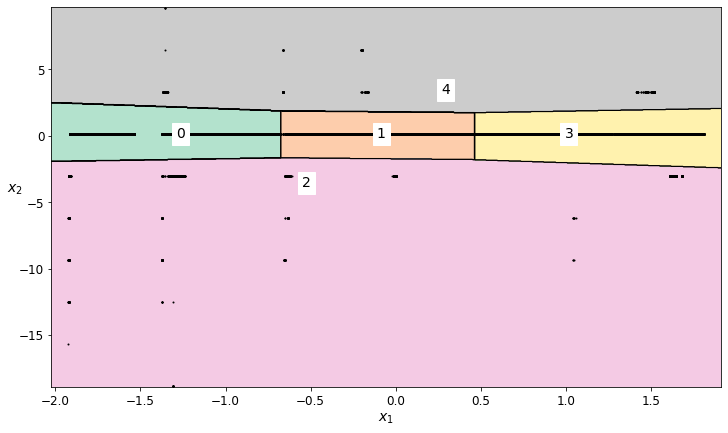
find outliers for the Scaled Longitude feature

field_to_analyze = 'Scaled Longitude'
number_of_clusters = 5


# Impute the data 
scaled_longitude_kmeans_data_imputed = transform_data_for_kmeans(scaled_data, field_to_analyze)

# Train the K-means model
scaled_longitude_kmeans = KMeans(n_clusters=number_of_clusters, random_state=41)

scaled_longitude_cluster_labels = scaled_longitude_kmeans.fit_predict(scaled_longitude_kmeans_data_imputed)

# Plot the decision boundaries
plt.figure(figsize=(12, 7))
plot_decision_boundaries(scaled_longitude_kmeans, scaled_longitude_kmeans_data_imputed)

# Based on the labeled regions from the decision boundary plot, decide which regions should be retained
scaled_longitude_regions_to_retain = [3,0,2]

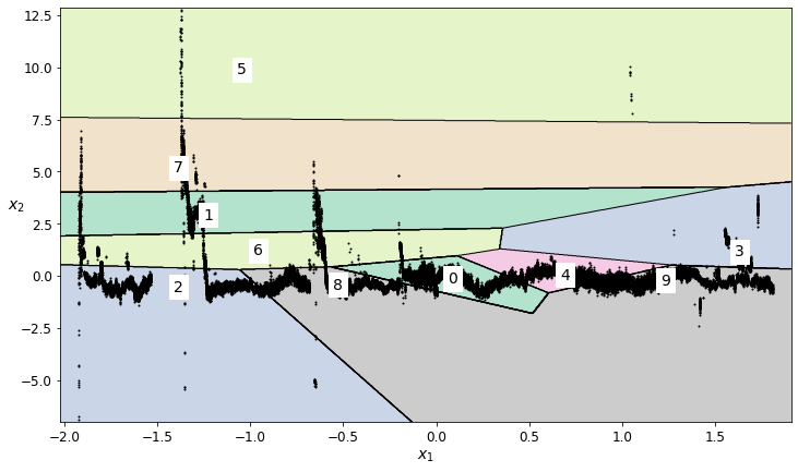
find outliers for the Vector Magnitude feature

field_to_analyze = 'Vector Magnitude'
number_of_clusters = 10

# Impute the data 
vector_magnitude_kmeans_data_imputed = transform_data_for_kmeans(scaled_data, field_to_analyze)

# Train the K-means model
vector_magnitude_kmeans = KMeans(n_clusters=number_of_clusters, random_state=42)

vector_magnitude_cluster_labels = vector_magnitude_kmeans.fit_predict(vector_magnitude_kmeans_data_imputed)

# Plot the decision boundaries
plt.figure(figsize=(12, 7))
plot_decision_boundaries(vector_magnitude_kmeans, vector_magnitude_kmeans_data_imputed)

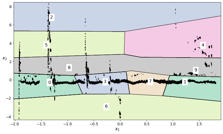
K-means did a nice job of locating the lower-noise signal for the derived Vector Magnitude feature - significantly better than for any of the individual un-combined features.

# Based on the labeled regions from the decision boundary plot, decide which regions should be retained
vector_magnitude_regions_to_retain = [4,1,6,3,7]

# Create a copy of the unfiltered scaled data object and selectively remove points

cleaned_kmeans_data = scaled_data

# Create a new column in the pandas object for the cluster labels for each dimension
cleaned_kmeans_data['scaled_height_kmeans'] = scaled_height_cluster_labels
cleaned_kmeans_data['scaled_longitude_kmeans'] = scaled_longitude_cluster_labels
cleaned_kmeans_data['scaled_latitude_kmeans'] = scaled_latitude_cluster_labels
cleaned_kmeans_data['vector_magnitude_kmeans'] = vector_magnitude_cluster_labels

# For each dimension, keep only the designated rows
cleaned_kmeans_data = cleaned_kmeans_data[cleaned_kmeans_data.scaled_height_kmeans.isin(scaled_height_regions_to_retain)]
cleaned_kmeans_data = cleaned_kmeans_data[cleaned_kmeans_data.scaled_longitude_kmeans.isin(scaled_longitude_regions_to_retain)]
cleaned_kmeans_data = cleaned_kmeans_data[cleaned_kmeans_data.scaled_latitude_kmeans.isin(scaled_latitude_regions_to_retain)]
cleaned_kmeans_data = cleaned_kmeans_data[cleaned_kmeans_data.vector_magnitude_kmeans.isin(vector_magnitude_regions_to_retain)]

Training the neural net

Training on unfiltered data

Generate the training set

# get the data in the proper format to train the Neural network

unfiltered_training_data, unfiltered_training_labels = get_neural_net_training_sets(scaled_data, 'Scaled Height', N_STEPS_TRAINING)

Create and train the neural network model

model = get_neural_net_model(N_STEPS_AHEAD)

history = model.fit(unfiltered_training_data, unfiltered_training_labels, epochs=20,)

Epoch 1/20
1/1 [==============================] - 4s 4s/step - loss: 0.2224 - last_time_step_mse: 0.2233
Epoch 2/20
1/1 [==============================] - 2s 2s/step - loss: 0.1985 - last_time_step_mse: 0.1986
Epoch 3/20
1/1 [==============================] - 2s 2s/step - loss: 0.1596 - last_time_step_mse: 0.1552
Epoch 4/20
1/1 [==============================] - 2s 2s/step - loss: 0.1034 - last_time_step_mse: 0.0994
Epoch 5/20
1/1 [==============================] - 2s 2s/step - loss: 0.0780 - last_time_step_mse: 0.0902
Epoch 6/20
1/1 [==============================] - 2s 2s/step - loss: 0.0599 - last_time_step_mse: 0.0714
Epoch 7/20
1/1 [==============================] - 2s 2s/step - loss: 0.0318 - last_time_step_mse: 0.0311
Epoch 8/20
1/1 [==============================] - 2s 2s/step - loss: 0.0174 - last_time_step_mse: 0.0173
Epoch 9/20
1/1 [==============================] - 2s 2s/step - loss: 0.0143 - last_time_step_mse: 0.0110
Epoch 10/20
1/1 [==============================] - 2s 2s/step - loss: 0.0120 - last_time_step_mse: 0.0097
Epoch 11/20
1/1 [==============================] - 2s 2s/step - loss: 0.0097 - last_time_step_mse: 0.0089
Epoch 12/20
1/1 [==============================] - 2s 2s/step - loss: 0.0097 - last_time_step_mse: 0.0088
Epoch 13/20
1/1 [==============================] - 2s 2s/step - loss: 0.0110 - last_time_step_mse: 0.0118
Epoch 14/20
1/1 [==============================] - 2s 2s/step - loss: 0.0103 - last_time_step_mse: 0.0133
Epoch 15/20
1/1 [==============================] - 2s 2s/step - loss: 0.0083 - last_time_step_mse: 0.0105
Epoch 16/20
1/1 [==============================] - 2s 2s/step - loss: 0.0072 - last_time_step_mse: 0.0066
Epoch 17/20
1/1 [==============================] - 2s 2s/step - loss: 0.0072 - last_time_step_mse: 0.0083
Epoch 18/20
1/1 [==============================] - 2s 2s/step - loss: 0.0071 - last_time_step_mse: 0.0053
Epoch 19/20
1/1 [==============================] - 2s 2s/step - loss: 0.0058 - last_time_step_mse: 0.0045
Epoch 20/20
1/1 [==============================] - 2s 2s/step - loss: 0.0046 - last_time_step_mse: 0.0049

Use the trained model to make prediction for N_STEPS_AHEAD time increments

Only use the number of points for the predictions that were used for training the neural net (plus the number of steps ahead that we want to predict)

number_of_records = N_STEPS_TRAINING + N_STEPS_AHEAD
truncated_scaled_data = scaled_data.head(number_of_records)

unfiltered_forecast_training_data, unfiltered_forecast_labels = get_neural_net_forecast_sets(truncated_scaled_data, 'Scaled Height', N_STEPS_TRAINING, N_STEPS_FORECAST, N_STEPS_AHEAD )

unfiltered_forecast_predictions = model.predict(unfiltered_forecast_training_data)[:, -1][..., np.newaxis]

Training on data filtered using Gaussian Mixtures

Generate the training set

cleaned_g_m_training_data, cleaned_g_m_training_labels = get_neural_net_training_sets(g_m_cleaned_data, 'Scaled Height', N_STEPS_TRAINING)

Create and train the neural network model

# Create a new set of training data based on the cleansed data
cleaned_model = get_neural_net_model(N_STEPS_AHEAD)

cleaned_history = cleaned_model.fit(cleaned_g_m_training_data, cleaned_g_m_training_labels, epochs=20,)

Epoch 1/20
1/1 [==============================] - 5s 5s/step - loss: 0.1053 - last_time_step_mse: 0.1057
Epoch 2/20
1/1 [==============================] - 2s 2s/step - loss: 0.0903 - last_time_step_mse: 0.0916
Epoch 3/20
1/1 [==============================] - 2s 2s/step - loss: 0.0678 - last_time_step_mse: 0.0680
Epoch 4/20
1/1 [==============================] - 2s 2s/step - loss: 0.0424 - last_time_step_mse: 0.0415
Epoch 5/20
1/1 [==============================] - 2s 2s/step - loss: 0.0382 - last_time_step_mse: 0.0425
Epoch 6/20
1/1 [==============================] - 2s 2s/step - loss: 0.0202 - last_time_step_mse: 0.0201
Epoch 7/20
1/1 [==============================] - 2s 2s/step - loss: 0.0108 - last_time_step_mse: 0.0116
Epoch 8/20
1/1 [==============================] - 2s 2s/step - loss: 0.0086 - last_time_step_mse: 0.0087
Epoch 9/20
1/1 [==============================] - 2s 2s/step - loss: 0.0065 - last_time_step_mse: 0.0053
Epoch 10/20
1/1 [==============================] - 2s 2s/step - loss: 0.0046 - last_time_step_mse: 0.0044
Epoch 11/20
1/1 [==============================] - 2s 2s/step - loss: 0.0047 - last_time_step_mse: 0.0044
Epoch 12/20
1/1 [==============================] - 2s 2s/step - loss: 0.0052 - last_time_step_mse: 0.0039
Epoch 13/20
1/1 [==============================] - 2s 2s/step - loss: 0.0044 - last_time_step_mse: 0.0039
Epoch 14/20
1/1 [==============================] - 2s 2s/step - loss: 0.0032 - last_time_step_mse: 0.0030
Epoch 15/20
1/1 [==============================] - 2s 2s/step - loss: 0.0029 - last_time_step_mse: 0.0026
Epoch 16/20
1/1 [==============================] - 2s 2s/step - loss: 0.0031 - last_time_step_mse: 0.0028
Epoch 17/20
1/1 [==============================] - 2s 2s/step - loss: 0.0030 - last_time_step_mse: 0.0048
Epoch 18/20
1/1 [==============================] - 2s 2s/step - loss: 0.0024 - last_time_step_mse: 0.0023
Epoch 19/20
1/1 [==============================] - 2s 2s/step - loss: 0.0019 - last_time_step_mse: 0.0018
Epoch 20/20
1/1 [==============================] - 2s 2s/step - loss: 0.0018 - last_time_step_mse: 0.0021

plt.figure(figsize=(14, 8))
plot_series(cleaned_g_m_training_data[0, :, 0], N_STEPS_TRAINING)

The plot above shows the cleaned/filtered data. Note that The large spikes have been completely removed.

Use the trained model to make prediction for N_STEPS_AHEAD time increments

number_of_records = N_STEPS_TRAINING + N_STEPS_AHEAD
truncated_g_m_cleaned_data = g_m_cleaned_data.head(number_of_records)

g_m_filtered_forecast_training_data, g_m_filtered_forecast_training_labels = get_neural_net_forecast_sets(truncated_g_m_cleaned_data, 'Scaled Height', N_STEPS_TRAINING-1, N_STEPS_FORECAST, N_STEPS_AHEAD)

g_m_filtered_forecast_predictions = cleaned_model.predict(g_m_filtered_forecast_training_data)[:, -1][..., np.newaxis]

Training on data filtered using K-Means

Generate the training set

kmeans_cleaned_training_data, kmeans_cleaned_training_labels = get_neural_net_training_sets(cleaned_kmeans_data, 'Scaled Height', N_STEPS_TRAINING)

#### Create and train the neural network model

# Create a new set of training data based on the cleaned data from the K-means algorithm
kmeans_cleaned_model = get_neural_net_model(N_STEPS_AHEAD)

kmeans_cleaned_history = kmeans_cleaned_model.fit(kmeans_cleaned_training_data, kmeans_cleaned_training_labels, epochs=20,)

Epoch 1/20
1/1 [==============================] - 5s 5s/step - loss: 0.1281 - last_time_step_mse: 0.1285
Epoch 2/20
1/1 [==============================] - 2s 2s/step - loss: 0.1109 - last_time_step_mse: 0.1125
Epoch 3/20
1/1 [==============================] - 2s 2s/step - loss: 0.0846 - last_time_step_mse: 0.0852
Epoch 4/20
1/1 [==============================] - 2s 2s/step - loss: 0.0528 - last_time_step_mse: 0.0524
Epoch 5/20
1/1 [==============================] - 2s 2s/step - loss: 0.0480 - last_time_step_mse: 0.0523
Epoch 6/20
1/1 [==============================] - 2s 2s/step - loss: 0.0271 - last_time_step_mse: 0.0269
Epoch 7/20
1/1 [==============================] - 2s 2s/step - loss: 0.0136 - last_time_step_mse: 0.0144
Epoch 8/20
1/1 [==============================] - 2s 2s/step - loss: 0.0105 - last_time_step_mse: 0.0109
Epoch 9/20
1/1 [==============================] - 2s 2s/step - loss: 0.0084 - last_time_step_mse: 0.0070
Epoch 10/20
1/1 [==============================] - 2s 2s/step - loss: 0.0059 - last_time_step_mse: 0.0062
Epoch 11/20
1/1 [==============================] - 2s 2s/step - loss: 0.0055 - last_time_step_mse: 0.0050
Epoch 12/20
1/1 [==============================] - 2s 2s/step - loss: 0.0064 - last_time_step_mse: 0.0048
Epoch 13/20
1/1 [==============================] - 2s 2s/step - loss: 0.0060 - last_time_step_mse: 0.0051
Epoch 14/20
1/1 [==============================] - 2s 2s/step - loss: 0.0043 - last_time_step_mse: 0.0041
Epoch 15/20
1/1 [==============================] - 2s 2s/step - loss: 0.0036 - last_time_step_mse: 0.0034
Epoch 16/20
1/1 [==============================] - 2s 2s/step - loss: 0.0038 - last_time_step_mse: 0.0036
Epoch 17/20
1/1 [==============================] - 2s 2s/step - loss: 0.0038 - last_time_step_mse: 0.0065
Epoch 18/20
1/1 [==============================] - 2s 2s/step - loss: 0.0033 - last_time_step_mse: 0.0032
Epoch 19/20
1/1 [==============================] - 2s 2s/step - loss: 0.0025 - last_time_step_mse: 0.0025
Epoch 20/20
1/1 [==============================] - 2s 2s/step - loss: 0.0022 - last_time_step_mse: 0.0024

Use the trained model to make prediction for N_STEPS_AHEAD time increments

number_of_records = N_STEPS_TRAINING + N_STEPS_AHEAD
truncated_kmeans_cleaned_data = cleaned_kmeans_data.head(number_of_records)

kmeans_filtered_forecast_training_data, kmeans_filtered_forecast_training_labels = get_neural_net_forecast_sets(truncated_kmeans_cleaned_data, 'Scaled Height', N_STEPS_TRAINING-1, N_STEPS_FORECAST, N_STEPS_AHEAD)

kmeans_filtered_forecast_predictions = kmeans_cleaned_model.predict(kmeans_filtered_forecast_training_data)[:, -1][..., np.newaxis]

Plots of unfiltered data

# Plot the entire training set 
plt.figure(figsize=(14, 8))
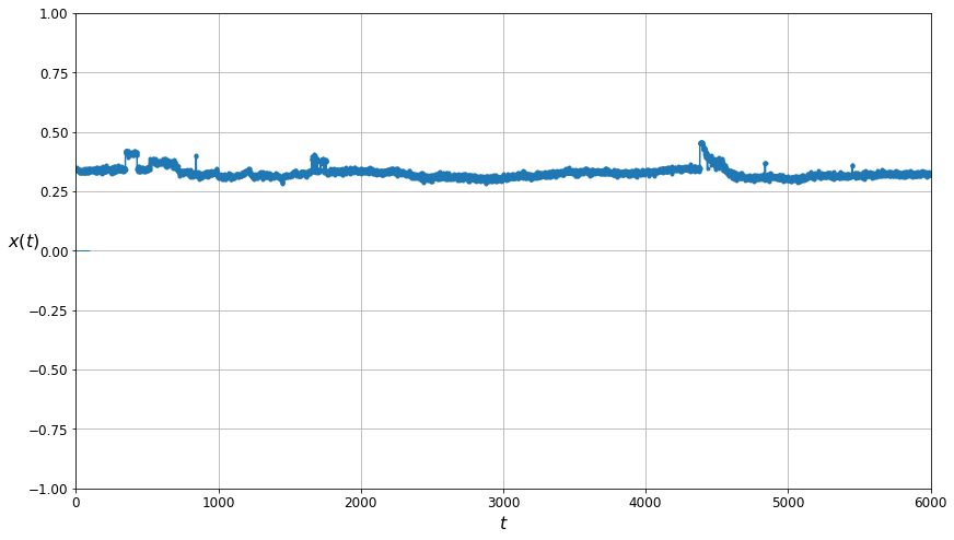
plot_series(unfiltered_training_data[0, :, 0], N_STEPS_TRAINING)
plt.show()

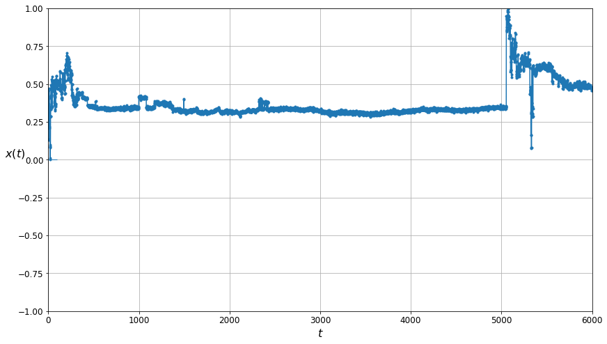
This is the plot for the unfiltered data. Note the large spikes!

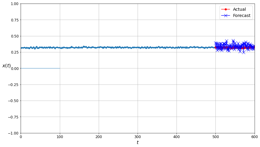
# Plot the last n_step_forecast
plt.figure(figsize=(14, 8))
plot_multiple_forecasts(unfiltered_forecast_training_data, unfiltered_forecast_labels, unfiltered_forecast_predictions, N_STEPS_FORECAST)

plt.show()

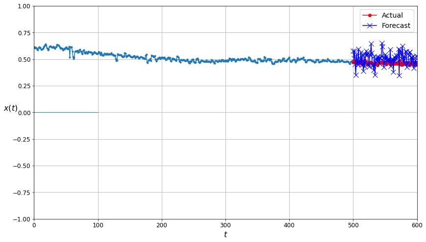
This plot compares how well the model did at predicting future time series points. The actual values from the time series are shown in red underneath the dark blue Xs indicating predictions made by the neural net trained on the unfiltered (uncleaned) data. Note that the forecast points aren’t particularly tightly clustered around the actual values.

Plots of Gaussian Mixtures cleaned / filtered data

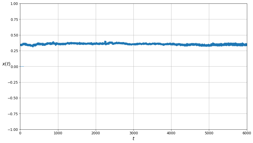
# Plot the entire training set for comparison
plt.figure(figsize=(14, 8))
plot_series(cleaned_g_m_training_data[0, :, 0], N_STEPS_TRAINING)

The plot of the data cleaned by the Gaussian Mixtures algorithm.

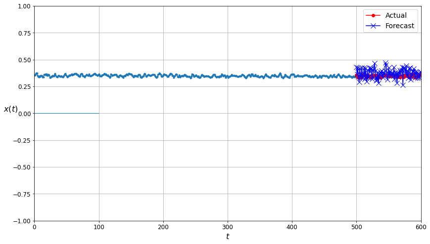
plt.figure(figsize=(14, 8))
plot_multiple_forecasts(g_m_filtered_forecast_training_data, g_m_filtered_forecast_training_labels, g_m_filtered_forecast_predictions, N_STEPS_FORECAST)

The comparison plot for the predictions made by the neural network trained on data filtered by the Gaussian Mixtures algorithm. The forecast points are much closer to the actual values than in the corresponding plot for the unfiltered data!

Plots of K-means cleaned / filtered data

# Plot the entire training set for comparison
plt.figure(figsize=(14, 8))
plot_series(kmeans_cleaned_training_data[0, :, 0], N_STEPS_TRAINING)

The plot of the data cleaned by the K-means algorithm. Note that visually it appears to be even more smooth than the plot of the data filtered using Gaussian Mixtures.

plt.figure(figsize=(14, 8))
plot_multiple_forecasts(kmeans_filtered_forecast_training_data, kmeans_filtered_forecast_training_labels, kmeans_filtered_forecast_predictions, N_STEPS_FORECAST)

The comparison plot for the predictions made by neural network trained on the data filtered by the K-mean algorithm. The forecast points are again closer to the actual values… but perhaps not quite as close as seen for the Gaussian Mixtures filtered data.

Compare the accuracy of the prediction made by the different trained models

The MSE of the unmodified data

mse = mean_squared_error(unfiltered_forecast_labels.flatten(), unfiltered_forecast_predictions.flatten())
mse

print("Mean squared error for the unmodified data: " + str(mse))

Mean squared error for the unmodified data: 0.0052735237

The MSE of the Gaussian Mixtures cleaned data

g_m_cleaned_mse = mean_squared_error(g_m_filtered_forecast_training_labels.flatten(), g_m_filtered_forecast_predictions.flatten())

print("Mean squared error for the data cleaned using Gaussian Mixtures: " + str(g_m_cleaned_mse))

Mean squared error for the data cleaned using Gaussian Mixtures: 0.0017369246

The MSE of the K-Means cleaned data

kmeans_cleaned_mse = mean_squared_error(kmeans_filtered_forecast_training_labels.flatten(), kmeans_filtered_forecast_predictions.flatten())

print("Mean squared error for the data cleaned using K-Means: " + str(kmeans_cleaned_mse))

Mean squared error for the data cleaned using K-Means: 0.0023650725

Percent improvement in neural network predictions

g_m_diff = (g_m_cleaned_mse/mse)*100
kmeans_diff = (kmeans_cleaned_mse/mse)*100

print("\n\nFor this run, the removal of the identified data points  results in a ")
print(str(round(100-g_m_diff)) + "% (Gaussian Mixtures)")
print(str(round(100-kmeans_diff)) + "% (K-means)")
print("reduced error rate in predicting values using the trained neural net\n")

For this run, the removal of the identified data points  results in a 
67% (Gaussian Mixtures)
55% (K-means)
reduced error rate in predicting values using the trained neural net

Both the Gaussian Mixtures and the K-means approach seem to significantly improve the prediction accuracy of the neural networks.

References

Daniels, M. D., Kerkez, B., Chandrasekar, V., Graves, S., Stamps, D. S., Martin, C., Dye, M., Gooch, R., Bartos, M., Jones, J., Keiser, K., 2016, Cloud-Hosted Real-time Data Services for the Geosciences (CHORDS) software (Version 0.9). UCAR/NCAR - Earth Observing Laboratory. https://doi.org/10.5065/d6v1236q

Kerkez, B., Daniels, M., Graves, S., Chandrasekar, V., Keiser, K., Martin, C., … Vernon, F. (2016). Cloud Hosted Real‐time Data Services for the Geosciences (CHORDS). Geoscience Data Journal, 3(1), 4–8. doi:10.1002/gdj3.36

Stamps, D. S., Saria, E., Ji, K. H., Jones, J. R., Ntambila, D., Daniels, M. D., & Mencin, D. (2016). Real-time data from the Tanzania Volcano Observatory at the Ol Doinyo Lengai volcano in Tanzania (TZVOLCANO). UCAR/NCAR - Earth Observing Laboratory. https://doi.org/10.5065/d6p849bm

Géron, A. (2019). Hands-On Machine Learning with Scikit-Learn, Keras, and TensorFlow: Concepts, Tools, and Techniques to Build Intelligent Systems (2nd ed.). O’Reilly.

Wikipedia contributors. (2021, February 3). Feature (machine learning). Wikipedia. https://en.wikipedia.org/wiki/Feature_(machine_learning)#cite_note-ml-1

7. Toward autonomous detection of anomalous GNSS data via applied unsupervised artificial intelligence 8. Exploring Research Data Repositories with geoextent.