Volcanic activity detection and noise characterization using machine learning
Author(s)
Author1 = {“name”: “Myles Mason”, “affiliation”: “Virginia Tech”, “email”: “mylesm18@vt.edu”, “orcid”: “0000-0002-8811-8294”}
Author2 = {“name”: “John Wenskovitch”, “affiliation”: “Virginia Tech”, “email”: “jw87@vt.edu”, “orcid”: “0000-0002-0573-6442”}
Author3 = {“name”: “D. Sarah Stamps”, “affiliation”: “Virginia Tech”, “email”: “dstamps@vt.edu”,”orcid”: “0000-0002-3531-1752”}
Author4 = {“name”: “Joshua Robert Jones”, “affiliation”: “Virginia Tech”, “email”: “joshj55@vt.edu”, “orcid”: “0000-0002-6078-4287”}
Author5 = {“name”: “Mike Dye”, “affiliation”: “Unaffiliated”, “email”: “mike@mikedye.com”, “orcid”: ” 0000-0003-2065-870X”}
Purpose
This Jupyter notebook explores methods towards characterizing noise and eventually predicting volcanic activity for Ol Doinyo Lengai (an active volcano in Tanzania) with machine learning using the TZVOLCANO CHORDS portal. Machine learning is a powerful tool that enables the automatization of complex mathematical and analytical models. In this Jupyter notebook, the components are time, height, latitude, and longitude. The predicted component values are the following heights. This project uses Global Navigation Satellite System (GNSS) data from the EarthCube CHORDS portal TZVOLCANO (Stamps et al. 2016; Daniels et al., 2016; Kerkez et al., 2016), which is the online interface for obtaining open-access real-time positioning data collected around Ol Doinyo Lengai. The bulk of the project is the exploration of the data and later prediction of height points. The station that this project analyzes is OLO1 for days 12/16/2020 and 04/16/2021.
Technical contributions
The training of the models and analysis uses basic linear algebra and statistics
The main libraries used (NumPy and pandas) are both libraries for data manipulation and linear algebra
The TZVOLCANO CHORDS portal linked above is the location of the data
Implementation of Linear Regression for prediction on time-series data
Methodology
The desired data was imported and selected with a range of about five months. The user downloads data from the TZVOLCANO CHORDS portal as a geojson file (.JSON). Previously downloaded JSON’s are converted to a Dataframe for easy manipulation further in the project. The information is then visualized for better analysis and statistical metrics running. Sample data size is increased for the project; A second JSON is introduced at the beginning of the data processing and analysis, which will later be used for OLO1 to predict height data from OLO1 on 4/16/2021 using 12/16/2020. We set up four series objects from the original data frame to be used for inputs for machine learning algorithms. The data set up for a linear regression shows the difference in target vs. predicted data in scatter plot form. Finally, nine predictions are displayed graphically with adjusting the test size data to demonstrate the different day prediction positions.
Results
This notebook explored predicting height data from the TZVOLCANO CHORDS portal using Linear Regression from different days. It also evaluates how much test data is needed to best predict height data. We find that having 10% test data yields the best results for predictions with the Mean Squared Error of 8.325e-5% . For predictions from data inputted and predicted from a single day we find the 75% test data yields the best results with an average error of -1.074e-4 meters.
Funding
Award1 = {“agency”: “National Science Foundation EarthCube Program”, “award_code”: “1639554”, “award_URL”: https://www.nsf.gov/awardsearch/showAward?AWD_ID=1639554&HistoricalAwards=false }
Award2 = {“agency”: “Virginia Tech Academy of Integrated Sciences Hamlett Undergraduate Research Award”, “award_code”: “44672”, “award_URL”: “”}
Keywords
keywords=[“tzDF”, “Linear Regression”, “Concat”, “Transpose”,”Mean Squared Error(MSE)”]
Citation
Mason, Myles, John Wenskovitch, D. Sarah Stamps, Joshua Robert Jones, Mike Dye (2021), EC_01_Volcanic_activity_detection_and_noise_characterization_using_machine learning, EarthCube Annual Meeting.
Suggested next steps
Noise activity in the data set is a topic that should be explored. Noise exploration is crucial to the development of this project because understanding the noise and being able to filter and characterize noise will allow any day to be analyzed efficiently and for more reliable predictions of hazardous volcanic deformation. Future next steps would include applying more classifying algorithms such as DBSCAN to characterize the noise.
Acknowledgements
Virginia Tech Department of Geosciences
Alice and Luther Hamlet
Setup
Library import
# Data manipulation
import pandas as pd
import json
import numpy as np
import math
from datetime import datetime as dt


# Visualizations
%matplotlib inline
import matplotlib.pyplot as plt
import seaborn as sns

# Modeling
from sklearn.linear_model import LinearRegression
from sklearn.model_selection import train_test_split
from sklearn.metrics import mean_squared_error
Parameter definitions
tzDF: intial dataframe contains 12/06/2020 datatz2DF: secondary dataframe contains 04/16/2021 dataONE_THROUGH_TWENTY: array of values in tzDF[“measurements_height”] used for predictionTWO_THROUGH_TWENTY_ONE:array of values in tzDF[“measurements_height”] used for predictionTHREE_THROUGH_TWENTY_TWO: array of values in tzDF[“measurements_height”] used for predictionFOUR_THROUGH_TWENTY_THREE: array of values in tzDF[“measurements_height”] used for predictionDECEMBER_SERIES_X: inputted height for 12/16/2020 data for Linear RegressionDECEMBER_SERIES_Y: target height data for 12/16/2020APRIL_SERIES_X: inputted height data for 04/16/2021APRIL_SERIES_Y: target height data for 04/16/2021APRIL_PREDICTION’: Predicted values from the two days
Data import
The CHORDS notebook portal is where the data is acessed.
#Import for JSON files for manipulation
''' Both files are station one, but the first date is December 16,2020
    while the second date is April 16 2021.
'''
with open('OLO1_12_16_20.geojson', 'r', encoding="utf-8") as infile:
    tzList = json.load(infile)

with open('OLO1_4_16_21.geojson', 'r', encoding="utf-8") as infile:
    tz2List = json.load(infile)
Data processing and analysis
#Convert both JSON's into  a partially-flattened pandas DataFrame
tzDF =  pd.json_normalize(tzList["features"][0]["properties"]["data"], sep='_')
tz2DF =  pd.json_normalize(tzList["features"][0]["properties"]["data"], sep='_')
#Overview of numerical elements of the data
print(tzDF.describe())
tzDF
       measurements_lat  measurements_height  measurements_lon
count      5.990000e+03          5990.000000      5.990000e+03
mean       2.734205e+00           988.153415      3.595022e+01
std        2.869056e-13             0.020116      1.547341e-07
min        2.734205e+00           988.095000      3.595022e+01
25%        2.734205e+00           988.139000      3.595022e+01
50%        2.734205e+00           988.152000      3.595022e+01
75%        2.734205e+00           988.167000      3.595022e+01
max        2.734205e+00           988.226000      3.595022e+01
| time | test | measurements_lat | measurements_height | measurements_lon | |
|---|---|---|---|---|---|
| 0 | 2020-12-16T05:08:18Z | false | 2.734205 | 988.203 | 35.950217 |
| 1 | 2020-12-16T05:08:19Z | false | 2.734205 | 988.206 | 35.950217 |
| 2 | 2020-12-16T05:08:20Z | false | 2.734205 | 988.214 | 35.950217 |
| 3 | 2020-12-16T05:08:21Z | false | 2.734205 | 988.226 | 35.950217 |
| 4 | 2020-12-16T05:24:41Z | false | 2.734205 | 988.199 | 35.950217 |
| ... | ... | ... | ... | ... | ... |
| 5985 | 2020-12-17T04:48:44Z | false | 2.734205 | 988.139 | 35.950217 |
| 5986 | 2020-12-17T04:53:51Z | false | 2.734205 | 988.147 | 35.950217 |
| 5987 | 2020-12-17T04:53:52Z | false | 2.734205 | 988.132 | 35.950217 |
| 5988 | 2020-12-17T04:55:09Z | false | 2.734205 | 988.137 | 35.950217 |
| 5989 | 2020-12-17T04:59:54Z | false | 2.734205 | 988.147 | 35.950217 |
5990 rows × 5 columns
From the .describe call looking at our data frame, there does not seem to be much variation in columns measurements_lat and measurements_lon because the DataFrame is from a single day. The reason for choosing to explore the measurements_height column in this notebook is because of the hypothesis that the surface will uplift if there is magma reservoir inflation or the surface will subside if there is magma reservior deflation. From viewing the data frame, the time column is in a time series form with extra separator variables “T” and “Z” in the following two cells; we will convert the timestamp column into an integer form for easy manipulation.
Function to convert timestamp column of tzDF and tz2DF from time series to an integer for easy manipulation.
def timeconvertfunc(timestamp):
 #The format of tzDF["measurments_height] is in string form and timeseries so this method make it an integer"
  ts = pd.Timestamp(timestamp, tz=None).to_pydatetime()
  ts = 3600*ts.hour + 60*ts.minute + ts.second

  return ts
#Applying above method to the two data frames
tzDF["timeconvert"] = tzDF["time"].apply(timeconvertfunc)
tz2DF["timeconvert"] = tzDF["time"].apply(timeconvertfunc)
Visualization of basic statistics from measurements_height and linear regression
In the code block below the four series objects are partitions of the measurements_height column in the tzDF DataFrame. We create these partitions to feed into a linear regression model for predictions.
# Series from the first Data Frame

ONE_THROUGH_TWENTY = tzDF["measurements_height"].loc[1:21].values.reshape(-1,1)
TWO_THROUGH_TWENTY_ONE = tzDF["measurements_height"].loc[2:22].values.reshape(-1,1)
THREE_THROUGH_TWENTY_TWO =tzDF["measurements_height"].loc[3:23].values.reshape(-1,1)
FOUR_THROUGH_TWENTY_FOUR = tzDF["measurements_height"].loc[4:24].values.reshape(-1,1)

#Linear Regression model on columns 1-20 and 2-21

lm = LinearRegression()
lm.fit(ONE_THROUGH_TWENTY ,TWO_THROUGH_TWENTY_ONE)
y_pred = lm.predict(ONE_THROUGH_TWENTY)
plt.xlabel("actual height(m)")
plt.ylabel("predicted height(m)")
plt.title("actual height vs predicted height")
plt.scatter(ONE_THROUGH_TWENTY,TWO_THROUGH_TWENTY_ONE)
plt.plot(ONE_THROUGH_TWENTY,y_pred,color="red")
plt.show()

#Method to round for sigfigs
def to_precision(x,p):
    x = float(x)
    if x == 0.:
        return "0." + "0"*(p-1)
    out = []
    if x < 0:
        out.append("-")
        x = -x
    e = int(math.log10(x))
    tens = math.pow(10, e - p + 1)
    n = math.floor(x/tens)
    if n < math.pow(10, p - 1):
        e = e -1
        tens = math.pow(10, e - p+1)
        n = math.floor(x / tens)
    if abs((n + 1.) * tens - x) <= abs(n * tens -x):
        n = n + 1
    if n >= math.pow(10,p):
        n = n / 10.
        e = e + 1
    m = "%.*g" % (p, n)
    if e < -2 or e >= p:
        out.append(m[0])
        if p > 1:
            out.append(".")
            out.extend(m[1:p])
        out.append('e')
        if e > 0:
            out.append("+")
        out.append(str(e))
    elif e == (p -1):
        out.append(m)
    elif e >= 0:
        out.append(m[:e+1])
        if e+1 < len(m):
            out.append(".")
            out.extend(m[e+1:])
    else:
        out.append("0.")
        out.extend(["0"]*-(e+1))
        out.append(m)

    return "".join(out)
print("The b value is",to_precision(lm.coef_[0][0],4))

print("The m value is",to_precision(lm.intercept_[0],4))


print("The R^2 value is",to_precision(lm.score(ONE_THROUGH_TWENTY,TWO_THROUGH_TWENTY_ONE),4),)
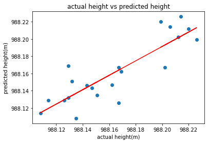
The b value is 0.8366
The m value is 161.5
The R^2 value is 0.7395
From the above model using the first through the twentieth column and second, through the twenty-second column, we yield a Coefficient of Correlation (R^2) value of about 0.74, which shows a positive correlation between the two inputs. So about 36% of the variation is residing in the residual.
Initiate Linear Regression
lm = LinearRegression()
lm.fit(TWO_THROUGH_TWENTY_ONE ,THREE_THROUGH_TWENTY_TWO)
y_pred1 = lm.predict(TWO_THROUGH_TWENTY_ONE)
plt.scatter(TWO_THROUGH_TWENTY_ONE,THREE_THROUGH_TWENTY_TWO)
plt.plot(TWO_THROUGH_TWENTY_ONE,y_pred1,color="green")
plt.xlabel("actual height(m)")
plt.ylabel("predicted height(m)")
plt.title("actual height vs predicted height")
plt.show()


print("This is the b value",to_precision(lm.coef_[0][0],4))
print("This is the m value",to_precision(lm.intercept_[0],4))
print("This is the R^2",to_precision(lm.score(TWO_THROUGH_TWENTY_ONE,THREE_THROUGH_TWENTY_TWO),4))
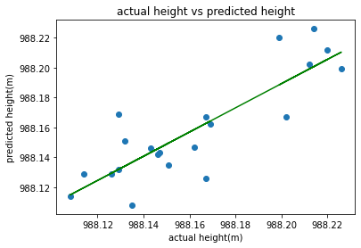
This is the b value 0.8102
This is the m value 187.5
This is the R^2 0.7257
From the above model using the first through the twentieth column and the second through the twenty-second column, we yield a Coefficient of Correlation (R^2) value of about 0.72, which shows a positive correlation between the two inputs. So about 38% of the variation is residing in the residual.
Linear Regression from single day
The following code chunk uses Linear Regression (specifically with rows of height measurement) for one_Through_Twenty,two_Through_Twenty_One, and three_Through_Twenty_Two. The data frame used for the model is tzDF, and we display the predicted values versus actual values.
#Set up series object for partions in the dataframe
ONE_THROUGH_TWENTY = tzDF["measurements_height"].loc[1:21]
TWO_THROUGH_TWENTY_ONE= tzDF["measurements_height"].loc[2:22]
THREE_THROUGH_TWENTY_TWO =tzDF["measurements_height"].loc[3:23]
FOUR_THROUGH_TWENTY_THREE = tzDF["measurements_height"].loc[4:24]

#Renaming the series objects
ONE_THROUGH_TWENTY.rename({"measurements_height":"w"},axis =1,inplace=True)
TWO_THROUGH_TWENTY_ONE.rename({"measurements_height":"x"},axis =1,inplace=True)
THREE_THROUGH_TWENTY_TWO.rename({"measurements_height":"y"},axis =1,inplace=True)
FOUR_THROUGH_TWENTY_THREE.rename({"measurements_height":"z"},axis =1,inplace=True)

#Concating the series objects to one dataframe, result_DF
result_DF = pd.concat([ONE_THROUGH_TWENTY,TWO_THROUGH_TWENTY_ONE,THREE_THROUGH_TWENTY_TWO,FOUR_THROUGH_TWENTY_THREE],axis=1)
result_DF

#Modefying dataframe by shifting the coulmns up
result_DF.iloc[:,1] = result_DF.iloc[:,1].shift(-1)
result_DF.iloc[:,2] = result_DF.iloc[:,2].shift(-2)
result_DF.iloc[:,3] = result_DF.iloc[:,3].shift(-3)

#Aligning all coulmns of the data frame together
result_DF = result_DF.dropna()
result_DF = result_DF.transpose()
result_DF

#Linear Regression on all rows and 1-19 coulmns
lm = LinearRegression()
x = result_DF.iloc[:,0:20]
y = result_DF.iloc[:,20]
lm.fit(x,y)
y_pred1 = lm.predict(x)
plt.scatter(y,y_pred1)
plt.xlabel("actual height(m)")
plt.ylabel("predicted height(m)")
plt.title("actual height vs predicted height")
plt.show()
#REMOVE CODE
#print("This is the b value",lm.coef_,)
#print("This is the m value",lm.intercept_)
#print("This is the R^2",lm.score(x,y))
print(y-y_pred1)
type(FOUR_THROUGH_TWENTY_THREE)
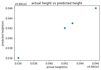
measurements_height    0.0
measurements_height    0.0
measurements_height    0.0
measurements_height    0.0
Name: 21, dtype: float64
pandas.core.series.Series
From the above graph, all points are predicted as the values overlap graphically with a b value of 0.0194. The height difference is zero. We will now increase the sample size of the data.
Method to increase sample size for the model
The method below takes in a data frame, goes into measurement height, and gets the first through nineteenth values in the height data frame. The first and nineteenth values are increased by one thousand times. The Data frame is transposed into columns then added to an empty list to be concatenated into a data frame.
#Making an empty list to store coulmn values
empty_list = []
def make_list(DataFrame):
    i = 0
    for i in range(1000):
        change = tzDF["measurements_height"].iloc[i+1:i+21].to_frame().transpose()
        #Names of the columns
        change.columns = ["history_1","history_2","history_3","history_4","history_5",
                          "history_6","history_7","history_8","history_9","history_10",
                          "history_11","history_12","history_13","history_14","history_15",
                          "history_16","history_17","history_18","history_19","history_20"]
        change.index = [i]
        empty_list.append(change)
    return empty_list
# List of all columns values
tzDF_list = make_list(tzDF["measurements_height"])
tzDF_two_list = make_list(tz2DF["measurements_height"])

#List iteration to combine all elements in list
finalDF = pd.concat([m for m in tzDF_list])
finalDF_two =  pd.concat([m for m in tzDF_two_list])
finalDF_two
| history_1 | history_2 | history_3 | history_4 | history_5 | history_6 | history_7 | history_8 | history_9 | history_10 | history_11 | history_12 | history_13 | history_14 | history_15 | history_16 | history_17 | history_18 | history_19 | history_20 | |
|---|---|---|---|---|---|---|---|---|---|---|---|---|---|---|---|---|---|---|---|---|
| 0 | 988.206 | 988.214 | 988.226 | 988.199 | 988.220 | 988.212 | 988.202 | 988.167 | 988.167 | 988.126 | 988.129 | 988.132 | 988.151 | 988.135 | 988.108 | 988.114 | 988.129 | 988.169 | 988.162 | 988.147 |
| 1 | 988.214 | 988.226 | 988.199 | 988.220 | 988.212 | 988.202 | 988.167 | 988.167 | 988.126 | 988.129 | 988.132 | 988.151 | 988.135 | 988.108 | 988.114 | 988.129 | 988.169 | 988.162 | 988.147 | 988.143 |
| 2 | 988.226 | 988.199 | 988.220 | 988.212 | 988.202 | 988.167 | 988.167 | 988.126 | 988.129 | 988.132 | 988.151 | 988.135 | 988.108 | 988.114 | 988.129 | 988.169 | 988.162 | 988.147 | 988.143 | 988.146 |
| 3 | 988.199 | 988.220 | 988.212 | 988.202 | 988.167 | 988.167 | 988.126 | 988.129 | 988.132 | 988.151 | 988.135 | 988.108 | 988.114 | 988.129 | 988.169 | 988.162 | 988.147 | 988.143 | 988.146 | 988.142 |
| 4 | 988.220 | 988.212 | 988.202 | 988.167 | 988.167 | 988.126 | 988.129 | 988.132 | 988.151 | 988.135 | 988.108 | 988.114 | 988.129 | 988.169 | 988.162 | 988.147 | 988.143 | 988.146 | 988.142 | 988.136 |
| ... | ... | ... | ... | ... | ... | ... | ... | ... | ... | ... | ... | ... | ... | ... | ... | ... | ... | ... | ... | ... |
| 995 | 988.100 | 988.106 | 988.131 | 988.121 | 988.129 | 988.129 | 988.146 | 988.148 | 988.131 | 988.130 | 988.145 | 988.112 | 988.127 | 988.140 | 988.114 | 988.122 | 988.151 | 988.164 | 988.140 | 988.143 |
| 996 | 988.106 | 988.131 | 988.121 | 988.129 | 988.129 | 988.146 | 988.148 | 988.131 | 988.130 | 988.145 | 988.112 | 988.127 | 988.140 | 988.114 | 988.122 | 988.151 | 988.164 | 988.140 | 988.143 | 988.146 |
| 997 | 988.131 | 988.121 | 988.129 | 988.129 | 988.146 | 988.148 | 988.131 | 988.130 | 988.145 | 988.112 | 988.127 | 988.140 | 988.114 | 988.122 | 988.151 | 988.164 | 988.140 | 988.143 | 988.146 | 988.132 |
| 998 | 988.121 | 988.129 | 988.129 | 988.146 | 988.148 | 988.131 | 988.130 | 988.145 | 988.112 | 988.127 | 988.140 | 988.114 | 988.122 | 988.151 | 988.164 | 988.140 | 988.143 | 988.146 | 988.132 | 988.133 |
| 999 | 988.129 | 988.129 | 988.146 | 988.148 | 988.131 | 988.130 | 988.145 | 988.112 | 988.127 | 988.140 | 988.114 | 988.122 | 988.151 | 988.164 | 988.140 | 988.143 | 988.146 | 988.132 | 988.133 | 988.117 |
2000 rows × 20 columns
Increased data points for linear regression
Below we will take the freshly made data frame finalDF with 200 rows x 20 columns, put the data into a linear regression utilizing the train test split module from the sci-kit library. The test sizes of 35, 55, and 75 are used for variability. The x is all of the rows in the new data frame and columns 1-19, while the or output is all of the rows and the 19th column that we are predicting.
35% Test Data demonstration
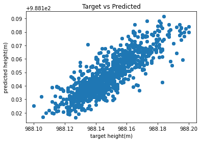
def make_prediction(DataFrame,number):
    input_Data = finalDF.iloc[:,0:19]
    target_Data = finalDF.iloc[:,19]
    lm = LinearRegression()
    lm.fit(input_Data,target_Data)
    y_pred1 = lm.predict(input_Data)
    plt.scatter(target_Data,y_pred1)
    plt.xlabel("target height(m)")
    plt.ylabel("predicted height(m)")
    plt.title("Target vs Predicted")
    plt.scatter
    # x axis is actual height and y is what lm model is predicting in scatter
    X_train, X_test, y_train, y_test = train_test_split(input_Data, target_Data,test_size = number, random_state=50)
    model = lm.fit(X_train,y_train)
    prediction = lm.predict(X_test)
    #Series of the difference of the test the leng
    error_Series = y_test-prediction
    #average
    average_Difference = sum(error_Series/len(error_Series))
    #print(average_Difference)
    print(to_precision(average_Difference,4))

make_prediction(tzDF,0.35)
-2.296e-4

When y_test-y_predicition, we get an average difference of -0.0003 from the model’s actual and predicted values in the above cell. From the outliers in the plot, we can view the noise graphically.
55% Test Data demonstration
#Function Call for 55% test data dem
make_prediction(tzDF,0.55)
-3.078e-4
In the above cell, when y_test-y_predicition, we get an average difference of -0.00030778063659289 from the model’s actual and predicted values.
75% Test Data demonstration
#Function Call for 75% test data dem
make_prediction(tzDF,0.75)
-1.074e-4

In the above cell when y_test-y_predicition we get an average difference of -0.0001 from the model’s actual and predicted values.
Using one day’s data to predict a different day’s data
The demonstrations below utilize the second data frame now named finalDF_two. The December 16, 2020 dates data will be trained to predict the April 16, 2020 dates data. The test size increases by ten percent in the range of 20-90 for variability. We will be using the Mean Squared value that shows the error for linear regression to view the model’s accuracy.
Prediction from 10% test size data
def different_Day_Prediction(DataFrame,number):
DECEMBER_SERIES_X = finalDF.iloc[:,0:19]
DECEMBER_SERIES_Y = finalDF.iloc[:,19]
APRIL_SERIES_X = finalDF_two.iloc[:,0:19]
APRIL_SERIES_Y= finalDF_two.iloc[:,19]
lm.fit(DECEMBER_SERIES_X,DECEMBER_SERIES_Y)
y_pred1 = lm.predict(DECEMBER_SERIES_X)
#train_test_split_module
X_train, X_test, y_train, y_test = train_test_split(DECEMBER_SERIES_X, APRIL_SERIES_Y, test_size=number,random_state=50)
model = lm.fit(X_train,y_train)
model.intercept_
model.coef_
#setting the predicition variable
APRIL_PREDICTION = model.predict(APRIL_SERIES_X)
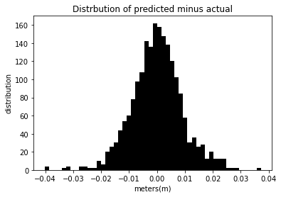
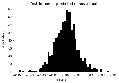
#50 bins were picked for all of the models below
#Distrubution of Errors pred vs actual
plt.hist(APRIL_PREDICTION-APRIL_SERIES_Y,bins = 50,color ="black")
plt.xlabel("meters(m)")
plt.ylabel("distribution")
plt.title("Distrbution of predicted minus actual")
plt.show()
#Displaying Mean Squared Error
twenty_MSE = mean_squared_error(APRIL_SERIES_Y,APRIL_PREDICTION)
print("The mean squared error for this model is",to_precision(twenty_MSE,4),"%.")
different_Day_Prediction(tzDF,.1)

The mean squared error for this model is 8.325e-5 %.
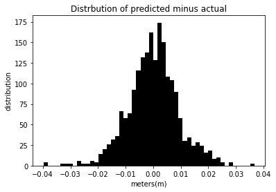
Prediction from 20% test size data
In the cell below, december_Series_X and decemeber_Series_Y will be the data that is used to train the model. April_Series_X and april_Series_Y will be the different days and data that we predict it points from. We will display a histogram to view the error distribution between the actual and predicted data as well as
different_Day_Prediction(tzDF,.2)

The mean squared error for this model is 8.344e-5 %.
In the above cell, the histogram displayed displays the error from the prediction minus the series. Most of the distribution of the data is centered around zero, indicating the performance of the model. The MSE is extremely low, showing the accuracy of the model.
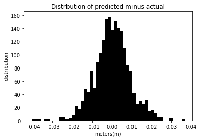
Prediction from 30% test size data
In the cell below our we will be inputting in 30% test data.
different_Day_Prediction(tzDF,.3)

The mean squared error for this model is 8.354e-5 %.
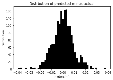
Prediction from 40% test size data
different_Day_Prediction(tzDF,.4)
The mean squared error for this model is 8.383e-5 %.
Prediction from 50% test size data
different_Day_Prediction(tzDF,.5)
The mean squared error for this model is 8.383e-5 %.
Prediction from 60% test size data
different_Day_Prediction(tzDF,.6)

The mean squared error for this model is 8.487e-5 %.
Prediction from 70% test size data
different_Day_Prediction(tzDF,.7)
The mean squared error for this model is 8.563e-5 %.
Prediction from 80% test size data
different_Day_Prediction(tzDF,.8)
The mean squared error for this model is 8.615e-5 %.
Prediction from 90% test size data
different_Day_Prediction(tzDF,.9)
The mean squared error for this model is 8.956e-5 %.
The mean square error for the above models is deficient, showing the success of inputting in height data for one day and predicting height data from another day.
Results
With this notebook we explored the use of machine learning for predictive analytics applied to vertical surface motions at an active volcano in Tanzania, Ol Doinyo Lengai. When training a model on one day and using that model to predict height values from another day, our lowest error was 8.325e-5 %. The future implications for this project and data are important because Ol Doinyo Lengai future eruption could cause distress for not only Tanzania, but other countries surrounding Tanzania. The ability to predict volcanic activity will be a valuable contribution to volcanic hazards assessment.
References
Daniels, Mike, Branko Kerkez, V. Chandrasekar, Sara Graves, D. Sarah Stamps, Charles Martin, Aaron Botnick, Michael Dye, Ryan Gooch, Josh Jones, Ken Keiser, Matthew Bartos, Thaovy Nguyen, Robyn Collins, Sophia Chen, Terrie Yang, Abbi Devins-Suresh (2016). Cloud-Hosted Real-time Data Services for the Geosciences (CHORDS) software (Version 1.0.1). UCAR/NCAR - EarthCube. https://doi.org/10.5065/d6v1236q
Kerkez, Branko, Michael Daniels, Sara Graves, V. Chandrasekar, Ken Keiser, Charlie Martin, Michael Dye, Manil Maskey, and Frank Vernon. “Cloud Hosted Real‐time Data Services for the Geosciences (CHORDS).” (2016), doi: 10.1002/gdj3.36.
GeÌ ron, Aureì lien. 2019. Hands-on Machine Learning with Scikit-Learn, Keras and TensorFlow: Concepts, Tools, and Techniques to Build Intelligent Systems. 2nd ed. CA 95472: O’Reilly.
Stamps, D. S., Saria, E., Ji, K. H., Jones, J. R., Ntambila, D., Daniels, M. D., & Mencin, D. (2016). Real-time data from the Tanzania Volcano Observatory at the Ol Doinyo Lengai volcano in Tanzania (TZVOLCANO). UCAR/NCAR - EarthCube. https://doi.org/10.5065/D6P849BM